One of the main advantages of Excel spreadsheets is the ability to program the functionality of a specific document. As most people know from school computer science lessons, one of the main components that allows you to implement this in practice is logical operators. One of them is the IF statement, which provides for the execution of certain actions if specific conditions are met.
For example, if the value matches a certain one, then one label is displayed in the cell. If not, another one. Let's take a closer look at this effective tool in practice.
IF Function in Excel (General Information)
Any program, even if it is small, necessarily contains a sequence of actions called an algorithm. It might look like this:
- Check the entire column A for even numbers.
- If an even number is found, add such and such values.
- If an even number is not detected, then display the message “not detected”.
- Check the resulting number to see if it is even.
- If yes, then add it with all the even numbers selected in step 1.
And even if this is only a hypothetical situation, which is unlikely to be necessary in real life, the execution of any task necessarily implies the presence of a similar algorithm. Before using the IF function,
you need to have a clear idea in your head of what result you need to achieve.
Syntax of the IF function with one condition
Any function in Excel is performed using a formula. The pattern by which data must be passed to a function is called syntax. In the case of the IF
, the formula will be in this format.
=IF (Boolean_expression;value_if_true;value_if_false)
Let's look at the syntax in more detail:
- Logical expression. This is the actual condition that Excel checks for compliance or non-compliance with. Both numeric and text information can be checked.
- Value_if_true. The result that will be displayed in the cell if the data being checked meets the specified criterion.
- Value_if_false. The result that is displayed in the cell if the data being checked does not meet the condition.
Here is an example for clarity.
1
Here the function compares cell A1 with the number 20. This is the first point of the syntax. If the content is greater than this value, the value “greater than 20” is displayed in the cell where the formula was written. If the situation does not meet this condition, “less than or equal to 20.”
If you need to display a text value in a cell, you need to put it in quotes.
Here's another situation. To obtain the right to take the examination session, students must pass the test. The students managed to pass the test in all subjects, and now the last one remained, which turned out to be decisive. Our task is to determine which students are allowed to take the exams and which are not.
2
Since we need to check the text and not the number, the first argument specifies B2=”credit.”.
Syntax of an IF function with multiple conditions
Often, one criterion is not enough; the value must be checked for compliance with it. If you need to consider more than one option, you can nest IF
one into the other. You will get several nested functions.
To make it more clear, here is the syntax.
=IF(logical_expression, value_if_true, IF(logical_expression, value_if_true, value_if_false))
In this case, the function will check two criteria at once. If the first condition is true, the value obtained as a result of the operation in the first argument is returned. If not, the second criterion is checked.
Here's an example.
3
And using this formula (shown in the screenshot below) you can analyze the performance of each student.
4
As you can see, one more condition was added here, but the principle has not changed. This way you can check several criteria at once.
Instead of TRUE or FALSE, a number is entered in the first argument
Because the value FALSE is equivalent to 0, then the formulas =IF(0;"Budget exceeded";"OK!") or (if cell A1 contains the value 0) =IF(A1;"Budget exceeded";"OK!") will return OK!
If cell A1 contains any number other than 0, the formula will return Budget Exceeded. This approach is convenient when checking whether a cell value is equal to zero.
Note : To make sure that the logical value FALSE corresponds to 0, enter the formula =—A1=0. In A1, enter FALSE. The formula will return TRUE. Note that the logical value FALSE corresponds exactly to 0, but is not equal to 0, because the formula =A1=0 will return FALSE, therefore the logical value FALSE is not equal to 0. Iron logic!
Note : The double negation "-" is simply a mathematical operation that converts a Boolean expression into a numeric expression, but does not change the value itself. Double negation can be replaced by addition with 0 or raising to the first power: =(A1+0)=0.
How to extend the IF functionality using the AND and OR operators
From time to time, the situation arises to check for compliance with several criteria at once, rather than using logical nested operators, as in the previous example. To do this, use either the AND
or the
OR
, depending on whether several criteria or at least one of them must be met. Let's take a closer look at these criteria.
IF function with AND condition
Sometimes you need to check an expression against several conditions at once. To do this, use the AND function written in the first argument of the IF
. It works like this: if a is equal to one and a is equal to 2, the value will be c.
IF function with OR condition
The OR function works in a similar way, but in this case, only one of the conditions needs to be true. A maximum of 30 conditions can be checked this way.
Here are options on how you can use the AND
and
OR
as an argument to the
IF
.
5 6
The simplest application example.
Let's say you work for a company that sells chocolate in several regions and deals with many customers.
We need to distinguish between sales that occurred in our region and those that were made abroad. To do this, you need to add one more attribute to the table for each sale - the country in which it occurred. We want this attribute to be created automatically for each record (that is, row).
The IF function will help us with this. Let's add the “Country” column to the data table. The West region is local sales (“Local”), and the remaining regions are foreign sales (“Export”).
Comparing data in two tables
From time to time you have to compare two similar tables. For example, a person works as an accountant and he needs to compare two reports. There are other similar tasks, such as comparing the cost of goods from different batches, student grades for different periods, and so on.
To compare two tables, use the COUNTIF
. Let's look at it in more detail.
Let's say we have two tables containing the technical specifications of two food processors. And we need to compare them and highlight the differences in color. This can be done using conditional formatting and the COUNTIF
.
Our table looks like this.
7
We select a range corresponding to the technical characteristics of the first food processor.
After this, you should click on the following menus: Conditional formatting - create a rule - use a formula to determine the cells to be formatted.
8
In the form of a formula for formatting, write the function =COUNTIF
(compared range; first cell of first table)=0. A table with the features of the second food processor is used as a comparison range.
9
You need to make sure that the addresses are absolute (with a dollar sign in front of the row and column names). You need to add =0 after the formula so that Excel looks for exact values.
After this, you need to set the formatting of the cells. To do this, next to the sample you need to click on the “Format” button. In our case, we use fill because it is most convenient for these purposes. But you can choose any formatting you want.
10
We assigned the column name as the range. This is much more convenient than entering the range manually.
SUMIF function in Excel
Now let's move on to the varieties of the IF
, which will help you replace two points of the algorithm at once.
The first one is SUMIF,
which adds two numbers that meet a certain condition. For example, we are faced with the task of determining how much money we need to pay per month to all sellers. For this it is necessary.
- Add a row with the total income of all sellers and click on the cell in which the result will be located after entering the formula.
- Find the fx button, which is located next to the line for formulas. Next, a window will appear where you can search for the required function. After selecting the operator, you need to click the “OK” button. But manual entry is always possible.
11 - Next, a window for entering function arguments will appear. All values can be specified in the appropriate fields, and the range can be entered using the button next to them.
12 - The first argument is the range. This is where you enter the cells that need to be checked to see if they meet the criteria. If we talk about us, these are employee positions. Enter the range D4:D18. Or simply select the cells of interest.
- In the “Criteria” field, enter the position. In our case, it is the “seller”. As a summation range, we indicate those cells where employee salaries are listed (this can be done either manually or by selecting them with the mouse). Click “OK” and we get the ready-calculated wages of all employees who are sellers.
Agree that this is very convenient. Is not it?
Combining a text string and a calculated formula
To make the result returned by some calculation more understandable to your users, you can associate it with a text explanation. It will explain how the results should be assessed.
For example, you can use the following formula to return the current date:
=CONCATENATE("Today";TEXT(TODAY();"dd-mmm-yyyy"))
To ensure that calculations with this function always give correct results, remember the following simple rules:
- It requires at least one text argument to work.
- You can combine up to 255 elements in one formula, for a total of 8,192 characters.
- The result is always text, even if all the input elements are numbers.
- It doesn't recognize arrays. Each link must be listed separately. For example, you should write
=CONCATENATE(A1, A2, A3)
instead of
=CONCATENATE(A1:A3)
- If at least one of the arguments to the CONCATENATE function is invalid, the expression returns the error #VALUE!
SUMIFS function in Excel
This function allows you to determine the sum of values that meet multiple conditions. For example, we were given the task of determining the total wages of all managers working in the southern branch of the company.
We add a row where the final result will be, and insert the formula in the desired cell. To do this, click on the function icon. A window will appear in which you need to find the SUMIFS
. Next, select it from the list and the familiar window with arguments opens. But the number of these arguments is now different. This formula makes it possible to use an infinite number of criteria, but the minimum number of arguments is five.
You can only specify five arguments via the argument input dialog. If more criteria are needed, they will have to be entered manually using the same logic as the first two.
Let's look at the main arguments in more detail:
- Summation range. Cells that will be summed.
- Condition Range 1 is the range that will be checked to see if the specific criterion is met.
- Condition 1 is the actual condition.
- Condition 2 range is the second range that will be tested against the criterion.
- Condition 2 is the second condition.
The further logic is similar. As a result, we determined the salaries of all managers of the Southern Branch.
13
COUNTIF function in Excel
If you need to determine how many cells fall under a certain criterion, use the COUNTIF function.
Let's say we need to understand how many salespeople work in this organization:
- First, add a line indicating the number of sellers. After this, you need to click on the cell where the result will be displayed.
- After this, you need to click on the “Insert Function” button, which can be found in the “Formulas” tab. A window will appear containing a list of categories. We need to select the “Full alphabetical list” item. In the list we are interested in the formula COUNTIF.
After we select it, we need to click the “OK” button.
14 - After this, we have the number of salespeople employed in this organization. It was obtained by counting the number of cells in which the word “seller” is written. It's simple.
Combine with space, comma and other characters
Your worksheets may often require you to put elements together so that they contain commas, spaces, various punctuation marks, or other characters such as a hyphen or slash.
To do this, simply include the desired symbol in the union formula. Be sure to enclose this character in quotation marks, as shown in the following examples.
This is how you can concatenate with a space:
=CONCATENATE(A1; » «; B1) or =A1 & » » & B1
Concatenation separated by commas:
=CONCATENATE(A1; ", "; B1) or =A1 & ", " & B1
Connect with a hyphen:
=CONCATENATE(A1; "-"; B1) or =A1 & "-" & B1
The picture shows what the results might look like: