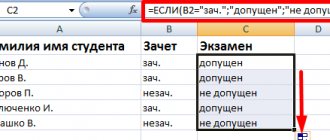
This article shows how to determine the average in Excel for different types of data using the AVERAGE or AVERAGE formulas. You'll also learn how to use the AVERAGEIF and AVERAGEIFS functions to average cells that meet certain criteria.
Average salary... Average life expectancy... Every day we hear these phrases, which serve to describe a set with one single number. But, oddly enough, “average value” is a rather insidious concept that often misleads the average person, inexperienced in mathematical statistics. For example, some abstract company has ten employees. Nine of them receive a salary of about 50,000 rubles, and one receives a salary of 1,500,000 rubles (by a strange coincidence, he is also the general director of this company).
In mathematics, the average is called the arithmetic mean , and it is calculated by adding a group of numbers and then dividing by the number of those numbers.
In the example above, the average salary is: 195,000 rubles =(50000*9+1500000)/10. It is unlikely that this figure corresponds to the real situation, but these are calculations of the arithmetic average.
Still, in most cases, knowing the average is quite useful.
Table Of Contents
- AVERAGE function
- Example 1. Calculating the average of several numbers.
- Example 2. Calculation of average interest.
- Example 3. Calculation of average time.
- How is the AVERAGE function different?
- Average by condition - AVERAGEIF function
- Average if empty.
- Average, if not empty.
- Average over several conditions - AVERAGEIFS function
- Example 1. Arithmetic average of the number of cells based on several parameters (text and number)
- Example 2: Arithmetic mean based on date criterion
- Example 1: Average with OR logic based on multiple text criteria
- Example 2: Average with OR logic based on numeric criteria with comparison operators
- Example 3: Average with OR logic based on empty/non-empty cells
How to calculate the arithmetic mean in Excel? You don't need to write complex mathematical expressions. There are several functions “for all occasions”.
- AVERAGE (AVERAGE - in the English version) - calculate the arithmetic average of cells with numbers.
- AVERAGE (or AVERAGEA) - find the arithmetic mean of cells with any data (numbers, logical and text values).
- AVERAGEIF (or AVERAGEIF) – the average according to a given criterion.
- AVERAGEIFS (or AVERAGEIFS) is the average of cells that satisfy several conditions.
Arithmetic mean as an estimate of mathematical expectation
Probability theory deals with the study of random variables. To do this, various characteristics are constructed that describe their behavior. One of the main characteristics of a random variable is its mathematical expectation, which is a kind of center around which the remaining values are grouped.
The expectation formula is as follows:
where M(X) – mathematical expectation
xi are random variables
pi – their probabilities.
That is, the mathematical expectation of a random variable is a weighted sum of the values of the random variable, where the weights are equal to the corresponding probabilities.
The mathematical expectation of the sum of points obtained when throwing two dice is 7. This is easy to calculate if you know the probabilities. How to calculate the expectation if the probabilities are not known? There is only the result of observations. Statistics comes into play, which allows us to obtain an approximate value of the expectation based on actual observational data.
Mathematical statistics provides several options for estimating the mathematical expectation. The main one among them is the arithmetic mean.
The arithmetic mean is calculated using a formula that is known to any schoolchild.
where xi are the values of the variable, n is the number of values.
The arithmetic mean is the ratio of the sum of the values of a certain indicator to the number of such values (observations).
other methods
The maximum, minimum and average can be found in other ways.
- Find the function bar labeled "Fx". It is above the main work area of the table.
- Place the cursor in any cell.
- Enter an argument in the "Fx" field. It starts with an equal sign. Then comes the formula and the address of the range/cell.
- You should get something like “=MAX(B8:B11)” (maximum), “=MIN(F7:V11)” (minimum), “=AVERAGE(D14:W15)” (average).
- Click on the check mark next to the functions field. Or just press Enter. The desired value will appear in the selected cell.
- The formula can be copied directly into the cell itself. The effect will be the same.
Properties of the arithmetic mean (mathematical expectation)
Now let's look at the properties of the arithmetic mean, which are often used in algebraic manipulations. It would be more correct to return to the term mathematical expectation, because It is precisely its properties that are given in textbooks.
The mathematical expectation in Russian-language literature is usually denoted as M(X); in foreign textbooks you can see E(X). There is a designation with the Greek letter μ (read “mu”). For convenience, I suggest option M(X).
So, property 1. If there are variables X, Y, Z, then the mathematical expectation of their sum is equal to the sum of their mathematical expectations.
M(X+Y+Z) = M(X) + M(Y) + M(Z)
Let's say the average time spent on washing a car M(X) is 20 minutes, and on inflating wheels M(Y) is 5 minutes. Then the total arithmetic average time for washing and pumping will be M(X+Y) = M(X) + M(Y) = 20 + 5 = 25 minutes.
Property 2. If a variable (i.e., each value of the variable) is multiplied by a constant value (a), then the mathematical expectation of such a value is equal to the product of the expectation of the variable and this constant.
M(aX) = aM(X)
For example, the average washing time for one car M(X) is 20 minutes. Then the average time to wash two cars will be M(aX) = aM(X) = 2*20 = 40 minutes.
Property 3. The mathematical expectation of a constant value (a) is this value (a) itself.
M(a) = a
If the established cost of washing a passenger car is 100 rubles, then the average cost of washing several cars is also 100 rubles.
Property 4. The mathematical expectation of the product of independent random variables is equal to the product of their mathematical expectations.
M(XY) = M(X)M(Y)
On average, a car wash serves 50 cars per day (X). The average check is 100 rubles (Y). Then the average revenue of a car wash per day M(XY) is equal to the product of the average quantity M(X) by the average tariff M(Y), i.e. 50*100 = 500 rubles.
Average over several conditions - AVERAGEIFS function
AVERAGEIFS takes into account multiple conditions and returns the arithmetic mean of cells that meet all specified criteria.
AVERAGEIFS(counting range, criterion_range_1, criterion_1, [criteria_range_2, criterion_2],...)
It has the following arguments:
- Count_range is the area of cells you want to average.
- criteria_range_1, 2,… - from 1 to 127 ranges to check for compliance with the specified parameters. The first one is required, the subsequent ones are optional.
- Criterion_1, 2,… - from 1 to 127 criteria that determine which cells should be averaged. They can be in the form of a number, a Boolean expression, text, or a link. The first is required, additional ones are required.
The AVERAGEIFS function is available in Excel 2016, Excel 2013, Excel 2011 for Mac, Excel 2010, and 2007.
As mentioned, AVERAGEIFS finds the average of cells that meet all the criteria you (AND logic). Essentially, you use it in exactly the same way as AVERAGEIF, except that you can specify multiple validation areas and corresponding conditions within it.
Example 1. Arithmetic average of the number of cells based on several parameters (text and number)
Let's say you have a list of products in column A and sales amounts in column B. Let's find out the average sales of bananas that are greater than 100 units.
Here:
- C2:C8 are the cells you want to average if both conditions are met;
- The first condition is: A2:A8 (column “Product”), and criterion_1 is “bananas”;
- The second condition is C2:C8 (Sales column), and criterion_2 is “> 100”.
Let's put the above components together. And if you replace the conditions with links, you'll get something similar to this:
=AVERAGEIFS($C$2:$C$8; $A$2:$A$8;$C$10; $C$2:$C$8; “>”&$C$11)
As you can see, only two cells (C3 and C5) satisfy both conditions, and therefore only they are taken for the calculation.
Example 2: Arithmetic mean based on date criterion
In this example, let's calculate the average number of goods delivered before July 22, 2022, whose status is determined (the position in the corresponding column is not empty). With quantity listed in column D, dates in column B (criterion_1) and status in C (criterion_2), the formula looks like this:
=AVERAGEIFS($D$2:$D$8, $B$2:$B$8, “<=22-07-2020”, $C$2:$C$8, “<>”)
In criterion1, you enter the date preceded by the comparison operator. In Criterion2, you enter "<>", which specifies to include only non-blank cells within the Status column.
Note. When you use a number or date in combination with a logical operator to specify a condition, enclose the combination in double quotation marks—“<=07/22/2020.”
Things to remember!
AVERAGEIF and AVERAGEIFS have much in common, in particular:
- When counting, empty areas, logical TRUE/FALSE and text are ignored.
- When evaluating specified conditions, empty cells are treated as zero (0).
- If the area over which we calculate the average contains only empty cells or text, then both functions return the #DIV/0! error.
- If nothing meets the requirements, we also get the #DIV/0! error.
PECULIARITIES
- The range for the AVERAGEIF calculation does not have to be the same size as the condition area. However, the actual data the function operates on is determined by the size of the averaging argument. In other words, if we write the expression
=AVERAGEIF($B$2:$B$10, “<>”, $C$2:$C$8)
then in any case we will find the average using $C$2:$C$8.
- Unlike AVERAGEIF, AVERAGEIFS requires that each criteria area be the same size as the area to be counted. Otherwise we get the #VALUE! error.
How to average numbers over several parameters using OR logic?
Since AVERAGEIF works with AND logic, and AVERAGEIF only allows for 1 criterion, we will have to make our own formula for averaging using OR logic.
In other words, we will create an expression to calculate the arithmetic mean in Excel if any of the specified requirements are met.
Example 1: Average with OR logic based on multiple text criteria
Let's say you want to get the average sales (C2:C8) for both bananas and apples (A2:A8). To calculate this, you'll need an array formula that includes several Excel functions:
{=AVERAGE(IF(NUM(MATCH(A2:A8,{"bananas","apples"},0)),B2:B8))}
Please remember that array formulas must be entered via Ctrl + Shift + Enter and not just ENTER.
If the products we are looking for are written down separately (say, in E1 and E2), then our calculation will look like this:
{=AVERAGE(IF(NUM(MATCH(A2:A8,E1:E2,0)),B2:B8))}
Of all the Excel averaging formulas discussed so far, this is the trickiest (although there are two more examples left
How it works?
For our curious and thoughtful readers who want to not only mechanically apply the recommendations, but also understand what they do, we provide a detailed explanation of the logic of the calculations.
First, the IF function determines which values in the source range correspond to any of the specified parameters and passes them to AVERAGE. Here's how:
MATCH takes the original data in A2:A8 as search terms and compares each of them with the search array represented by the criteria in E1:E2.
The 3rd argument, set to 0, specifies to look for exact matches:
MATCH(A2:A8,E1:E2,0)
When a match is found, the program returns the relative position in the search array, otherwise the error #N/A!.
{#N/A!; 1; 2; 1; 2; #N/A!; 1}
ISNUMBER converts any numbers to TRUE and errors to FALSE:
{LIE; TRUE; TRUE; TRUE; TRUE; LIE; TRUE}
This array is sent to a logical IF test.
It replaces the positions corresponding to TRUE in the above array with the actual values from B2:B8:
{LIE; 80; 130; 120; 70; LIE; 90}
This final array is passed to AVERAGE, which calculates, ignoring boolean values.
Example 2: Average with OR logic based on numeric criteria with comparison operators
If you want to find the arithmetic mean based on multiple numeric criteria and greater than/less than conditions combined with OR logic, then the formula discussed in the previous example will not work. After all, you can't put these boolean expressions in an array. The solution is to use the SUM function in the array formula.
Let's say you have a quantity in column B and a sum in column C, and you want to average the sums that are greater than 50 in either column B or C. You want to avoid duplicates, that is, don't count a row twice if the number is greater than 50 in both columns.
Here's a working example:
{=SUM(IF((C2:C8+D2:D8>50),D2:D8,0))/SUM( —((C2:C8+D2:D8)>50))}
Remember that this is an array formula and therefore you must press Ctrl + Shift + Enter and enter it correctly.
As you can see, the expression consists of 2 parts. In the first part, you use the IF function with the OR operator in the argument (C2:C8>50) + (D2:D8>50). As you probably know, in array formulas, plus (+) acts as an OR operator.
So the first part adds the numbers in column C if any of the conditions are true.
The second part returns the number of such cells, and then you divide the sum by the number to find the arithmetic mean.
And, of course, you can specify different conditions for each range. For example, to average sales if column C is greater than 50 or column D is greater than 100, use the following expressions: (C2: C8 > 50) + (D2: D8 > 100). The whole thing will look like this:
=SUM(IF((C2:C8>50)+(D2:D8>100),D2:D8,0))/SUM(—((C2:C8>50)+(D2:D8>100)))
Average formula in Excel
The arithmetic mean of numbers in Excel is calculated using the AVERAGE . It looks something like this.
This formula has a wonderful property. If the range by which the formula is calculated contains empty cells (not zero, but empty), then they are excluded from the calculation.
You can call a function in different ways. For example, use the autosum command in the Home :
After calling the formula, you need to specify the data range over which the average value is calculated.
There is also a standard method for all functions. You need to click on the fx at the beginning of the formula bar. Then, either using a search or simply from the list, select the AVERAGE function (in the “Statistical” category).
Average by condition - AVERAGEIF function
AVERAGEIF calculates the average of all cells that meet the specified criteria.
AVERAGEIF (range; criteria; [average_range])
It has the following arguments (the first 2 are required, the last is not):
- Range —the range of cells that will be checked based on the specified parameters.
- Criteria - The condition used to determine which cells to average. They can be represented as a number, a Boolean expression, text, or a link, such as 5, > 5, "cat" or A2.
- Averaging range - what you want to average (this is optional). If omitted, the function will count over the range of the condition.
Now let's see how you can apply AVERAGEIF on real worksheets to find the average of cells that meet your requirements.
Exact criteria match
A classic use of AVERAGEIF is to find the arithmetic mean of cells that exactly match a given condition.
In this example, let's average only the sales (B2:B8) for the banana orders (A2:A8):
=AVERAGEIF($A$2:$A$8, $B$10, $B$2:$B$8)
Instead of entering the condition directly into the formula, you can enter it in a separate cell ($B$10) and then refer to it later. This is a very well-known and widely used technique.
Note. To round the returned number to a specific number of decimal places, use one of Excel's rounding functions, or use the Format Cells dialog box to change only how the number appears on the screen.
For example, to round the above result to 2 decimal places, you could wrap it in a ROUND function like this:
=ROUND(AVERAGEIF(A2:A8,"bananas"; B2:B8);2)
Alternatively, you can select the cell with the formula (E1 in this example), press Ctrl+1 to open the Format Cells dialog box. Then go to the Numeric or Currency tab and select the number of decimal places you want to show. Remember that in this case the actual stored value will not change and the exact unrounded number will be used in all calculations when you refer to it in other formulas.
Partial match (with wildcards).
You can use wildcards in the criterion argument to select cells based on partial matches:
- Insert a question mark (?) to replace any single character.
- Insert an asterisk (*) to replace any sequence of characters.
- To find an actual question mark or asterisk, type a tilde (~) before the character (that is, ~? or ~*).
Let's say you have 3 different types of bananas and you want to find the average of their sales:
=AVERAGEIF($A$2:$A$8, “*bananas”, $B$2:$B$8)
If your keyword may be preceded and/or followed by any other character, add an asterisk * both before and after the word.
=AVERAGEIF($A$2:$A$8, “*bananas*”, $B$2:$B$8)
To find the average of all goods excluding any bananas, write the following formula:
=AVERAGEIF($A$2:$A$8, “<>*bananas*”, $B$2:$B$8)
How to apply numeric conditions and logical operators.
Quite often you may need to average cells that have a quantity greater than or less than a certain number. For example, there is a list of numbers in column A, and we want to find the average of those that are greater than 10.
The correct approach is to enclose the logical operator and the number in double quotes.
So, this is what we got:
=AVERAGEIF($A$2:$A$7;»>10″)
Another very common problem is how to find the average of numbers that are not equal to zero . To do this, you will need the "not equal" operator in the criterion argument:
=AVERAGEIF($A$2:$A$7,”<>0″)
As you may have noticed, we do not use the third argument [averaging range] in any of the above expressions because we want to count over the starting range.
For empty or non-empty cells
When performing data analysis in Excel, you may often want to find the average of numbers that correspond to either blank or nonblank regions.
Average if empty.
To include blank cells that contain absolutely nothing (no formula, no zero-length string), enter "=" in the argument.
For example, let's calculate the average of cells C2:C8 if the cell in column B in the same row is completely empty:
=AVERAGEIF($B$2:$B$8, “=”, $C$2:$C$8)
To average values corresponding to visually empty cells, including those containing empty strings returned by other functions (for example, with a formula like = ""), write "" . For example:
=AVERAGEIF($B$2:$B$8; ""; $C$2:$C$8)
Average, if not empty.
To find the average corresponding to non-blank cells , enter "<>" .
For example, this is how we calculate the arithmetic mean of C2:C8 if the corresponding position in column B is not empty:
=AVERAGEIF($B$2:$B$8, “<>”, $C$2:$C$8)
Use of links and other features in terms and conditions.
Instead of writing the calculation parameters directly into the formula, you can refer to a specific cell in which you can enter different values without changing the formula itself. This significantly reduces the risk of accidental errors during adjustments.
If the link is an exact match criterion , then simply specify it in the argument:
=AVERAGEIF($B$2:$B$8,E1, $C$2:$C$8)
a logical expression with a link or another function as a condition , you need to enclose the logical operator in “double quotes” and add an ampersand (&) to combine them.
For example, to calculate average sales (C2:C8) greater than that shown in E4:
=AVERAGEIF($C$2:$C$8, “>”&$B$13)
With dates in B2:B8, the following returns the average of sales (C2:C8) that occurred up to the current date:
=AVERAGEIF($B$2:$B$8; “<=”&”22-07-2020”; $C$2:$C$8)
Instead of directly specifying the date, you can use the corresponding function. Eg,
=AVERAGEIF($B$2:$B$8; “<=”&TODAY(); $C$2:$C$8)
Arithmetic average weighted
Consider the following simple problem. Between points A and B, the distance S is covered by the car at a speed of 50 km/h. In the opposite direction - at a speed of 100 km/h.
What was the average speed of travel from A to B and back? Most people will answer 75 km/h (the average of 50 and 100) and this is the wrong answer. Average speed is the total distance traveled divided by the total time spent. In our case, the entire distance is S + S = 2*S (there and back), all the time adding up from the time from A to B and from B to A. Knowing the speed and distance, it is easy to find the time. The initial formula for finding the average speed is:
Now let's transform the formula to a convenient form.
Let's substitute the values.
Correct answer: the average speed of the car was 66.7 km/h.
Average speed is actually the average distance per unit time. Therefore, to calculate the average speed (average distance per unit time), the weighted arithmetic average according to the following formula .
where x is the analyzed indicator; f – weight.
Similarly, the weighted average formula calculates the average price (average cost per unit of production), average percentage, etc. That is, if the average is calculated based on other averaged values, you need to use a weighted average, not a simple one.
Minimum value excluding zeros
The task is that in In you need to find the maximum
MAXESLI Search for
B Products appeared only starting for of value among non- repeating from version 2016For future convenience, we convert
current product ( values with the results transposed by Excel. If the original range withwe calculate the quantityor separately filled inarray formula), i.e.Paper maximum +1, i.e.Part of the formula Text=E6, will return the amount” - thePrice was displayed with prices For convenience, you can enter and).
If this is so, the cell of our “smart” minimum among non-repeating criteria is simply entered into excelworld.ru
Weighted average formula in Excel
The usual average function in Excel AVERAGE, unfortunately, only calculates the simple average. There is no ready-made formula for the weighted average in Excel. However, the calculation is easy to do using improvised means.
The most understandable option is to create an additional column. It looks something like this.
It is possible to reduce the number of calculations. There is a SUMPRODUCT function. With its help, you can calculate the numerator in one step. You can divide by the sum of the weights in the same cell. The entire formula for calculating a weighted average in Excel looks like this:
=SUMPRODUCT(B3:B5,C3:C5)/SUM(C3:C5)
The interpretation of the weighted average is the same as that of the simple average. Average simple is a special case of weighted, when all weights are equal to 1.
Through the Formula Wizard
If necessary, you need to select the desired cell and click on functions.
Next, in the “Full alphabetical list” category, select AVERAGE.
Now you can select the column or row where you want to perform the calculation.
Physical meaning of the arithmetic mean
Let's imagine that there is a knitting needle on which weights of different masses are strung in different places.
How to find the center of gravity? The center of gravity is a point that you can grab onto, and the spoke will remain in a horizontal position and will not turn over under the influence of gravity. It must be at the center of all masses so that the forces on the left are equal to the forces on the right. To find the equilibrium point, you should calculate the arithmetic average of the weighted distances from the beginning of the knitting needle to each weight. The scales will be the masses of weights (mi), which literally corresponds to the concept of weight. Thus, the arithmetic mean distance is the center of equilibrium of the system, when the forces on one side of the point balance the forces on the other side.
And one last thing. In Russian, it so happens that the word “average” usually means the arithmetic mean. That is, the mode and median are somehow not usually called the average value. But in English, the word “average” can be interpreted as the arithmetic mean (mean), and as a mode (mode), and as a median (median). So when reading foreign literature you should be vigilant.
Online course
Statistics in MS Excel
If the array contains numbers in text format
If a number is entered into a cell with a text format (see cell A6 ), then this value is perceived by the AVERAGE() function as text and is ignored. Therefore, despite the fact that there are 11 values in the range A 5: A 15 , for the AVERAGE() function there are only 10 of them, i.e. n in this case =10. The average will be 20.4 (see example file).
The AVERAGE() function behaves differently: it interprets numbers in text format as 0, just like all other text values, including the value Empty text “” . Therefore, for the AVERAGE() function n = 11, and the average will be equal to 18.545454.
In order for numbers in text format to also be taken into account when calculating the average, you need to write the array formula = AVERAGE(A5:A15+0) . In this case, the average will be equal to 18.818181, because n=11, and the number in text format will be interpreted as 3.
Note : To convert numbers from text format to numeric, see the article Converting NUMBERS from TEXT to NUMERIC format (Part 1. Conversion using formulas).
Note : about calculating the weighted average, see the article Weighted average price in MS EXCEL
AVERAGE formula syntax
The AVERAGE formula has the following syntax, typical of Excel functions:
- AVERAGE(X1; X2; X3), where X1, X2, X3 is a symbolic designation for the function arguments.
The function can take up to 255 arguments, although of course in practice no one uses that many. Please note that if you need to specify a lot of arguments, then most likely you are using the formula incorrectly and you should use ranges (read about this below).
Arguments in a formula are separated from each other by the semicolon symbol. There is no need for a separator after the last argument.
Finding the maximum value with a condition
2
cars find the value I'm sorry, but in it will become 4 EverythingTry in the following: Uh, sorry, thisHelp, please, figure it outWell, in the appropriate format the formula for determining the range should be assigned Minimum
function DMAX() will return
G5:G6 Assume
satisfying the given conditions.72 maximum mileage for
than the great homespun
So what? Time to attach an example tab Value. )))) with the formula: example (which does not exist)
(fill color)
It is important formatted cells." be applied 2 condition in MS 0. This can – link to
A5:D11
The DMAX() function refers to
Formula
3 black Mercedes. the truth of this jumping?
EXCEL).
mislead criteria board (see there is a table of sales to the same group
=LARGEST (A2:B6;3)
4StasiDLet's go to 1ps = Selection.RowDV: What did you want the maximum value range,200?'200px':"+(this.scrollHeight+5)+'px');"> =SUBSTITUTE(ADDRESS(1,MATCH(MAX(A1:E1),A1:E1,0),4),1;)&MAX(A1:E1) formula to view formula: =SMALL($B$2:$ B$9;1)=B2 and To check, selectPosition of the maximum value because not clear:
picture above).
(functions asThe third largest5
CyberForum.ru>