How to create a formula in Excel: a guide to Excel tables

Good afternoon.

Once upon a time, writing a formula in Excel on my own was something incredible for me. And even despite the fact that I often had to work in this program, I didn’t type anything except text...

As it turned out, most of the formulas are not complicated and can be easily worked with, even by a novice computer user. In this article, I would like to reveal the most necessary formulas with which you most often have to work...

So, let's begin…

2. Addition of values in rows (formula SUM and SUMIFS)
2.1. Addition with condition (with conditions)

3. Counting the number of rows that satisfy the conditions (COUNTIFS formula)

4. Search and substitution of values from one table to another (VLOOKUP formula)

5. Conclusion

Mathematical operators

One of the main advantages of Excel is that it allows you to perform calculations using mathematical formulas, making your spreadsheets more convenient and flexible.

The program is capable of performing not only simple tasks, but also very difficult calculations. First, let's look at the standard actions:

plus (+) - addition;
minus (-) - subtraction;
oblique stripe (/) - division;
star (*) - multiplication;
symbol of the roof of the “house” (^) - degree.

To create any Excel formula, you first need to put an equal sign (=).

For convenience, the program provides an option that allows you to perform mathematical operations in relation to cell numbers.

The idea is that the user uses specific addresses, and then Excel performs the calculations.

The use of the method provides advantages in the form of reducing the number of erasures and making changes easier.

With this in mind, we can summarize how to correctly compose the formula. To do this, put an equal sign in the desired cell, and then indicate the necessary actions, for example, B1+B2 or A1*A2.

Thank you!

We will contact you soon.

COUNT: Counting the number of values

COUNT function counts the number of cells in a specified range that contain numbers. For example, you have 9 product positions, and you need to find out how many of them were purchased. Select the required area with values and click “OK” - the function will display the result. In our case, everything could be calculated manually, but what to do if there are hundreds of such values? Correct - use the COUNT operation.

If you need to count the filled cells, use the COUNTA . It works on a similar principle, but returns the number of cells with values in a given range.

Simple formulas

As a rule, Excel users make do with simple mathematical operations using subtraction, addition, and other signs. We will begin the instructions by considering such calculations.

Rules for creating formulas

Any Excel user should be able to create formulas of varying complexity. This allows you to use the full potential of the program and make calculations with a large number of actions simple.

Let's give an example of a simple formula for adding two numbers. The algorithm is like this:

Select the cell where the final result should be (C3).
Put an equal sign. Please note that it appears not only in the cell, but also in the top line.
Specify the address of the section that should be first, for example, C1.
Place the sign you are interested in in a specific formula, for example, plus (+).
Enter the address of the column for the second number, for example, C2.
Check that you have the inscription = C1 + C2, press Enter.

Above we have provided a simple explanation for beginners to understand the general principle of calculations in Excel.

If ###### appears in the column where the formula was written, this indicates that the column is not wide enough. The resulting number simply does not fit into the specified line.

The convenience is that an Excel user can make edits to table data without adjusting the formula.

If you change the value in C1 or C2, the final parameter in C3 will also change. The disadvantage is that Excel does not check formulas for errors, so you need to control this point yourself.

Selecting with the mouse

To simplify your work, you can minimize the use of the keyboard and use the mouse button to enter the formula. Take the following steps:

Select the section in the table where the formula (B3) will be located.
Place an equal sign (=).
Click on the cell that should appear first in the calculations. For the current example B1. The number will be circled and the section number will appear in the final column.
Specify the action to be taken. Alternatively, click on multiplication (*).
Select the cell whose number should be second in the formula (B2). Please note that the required area will be outlined with a dotted line.
Click on Enter for the system to perform the calculation.

In the future, you can copy formulas to other cells so as not to transfer them several times.

Editing

There are situations when it is necessary to change an already made formula in Excel. The reason could be any - a revision of the calculation algorithm, an error or other problems.

To make edits, do the following:

Specify the section where changes need to be made. In our case this is C3.
Go to the formula bar at the top to make adjustments. Alternatively, you can click directly on the cell to take a look and make changes to the formula.
Enter new data and notice which cells are highlighted by the program. Be careful at this stage to avoid mistakes.
Press Enter and confirm your changes. For example, if previously the formula looked like C1+C2, it can be changed to C1-C2 or any other option. The main thing is that the indicated cells contain numbers.

If desired, you can mark the actions taken. To do this, press Esc on the keyboard or select the Cancel sign in the line with the formula.

To view specified arithmetic operations, you can do it easier - click on the Ctrl+' combination.

Useful links: Canvas online editor, TOP programs for screen recording, Paint to draw online without downloading.

SUMIF, COUNTIF, AVERAGEIF

Formula: =SUMMIF(range, condition, sum_range) =COUNTIF(range, condition)

=AVERAGEIF(range, condition, averaging_range)

English version: =SUMIF(range; condition; sum_range), =COUNTIF(range; condition), =AVERAGEIF(range; condition; averaging_range)

These formulas perform the corresponding functions - SUM, COUNT, AVERAGE, if the specified condition is met.

Formulas with several conditions - SUMIFS, COUNTIFS, AVERAGEIFS - perform the corresponding functions if all specified criteria are true.

Using the functions in the previous example, we can find out:

SUMIF – total income only for sellers who have met the quota.

AVERAGEIF – the average income of the seller if he fulfilled the norm.

COUNTIF – the number of sellers who have fulfilled the quota.

Complex formulas

There are situations when a simple action is not enough and you need to set a complex formula.

Here it is necessary to take into account the general rules for mathematical operations. They are simple.

Multiplication and division are done first. In this case, operations in brackets have priority over other actions.

Here is a version of the formula for cell C4. You can specify the following data in it (B2+B3)*0.3.

This means that the formula first sums the two indicators, and the resulting value is calculated with a percentage (30% is written as 0.3).

During calculations, Excel follows the specified order. First, the operations in parentheses are performed, and only then the multiplication is done.

When writing a complex formula, it is important to take into account the calculation rules, because otherwise the result will be erroneous. Using parentheses is the best way to specify the correct order of calculations.

Remember that Excel makes calculations based on the entered data and does not warn about errors. Check the correctness of your input yourself. The main thing is to correctly place the brackets and set the calculation priorities.

Program functions

One of the main features of Excel is the availability of special functions. Essentially, this is a formula that makes certain calculations taking into account given parameters. They are designed to speed up and simplify calculations of various levels of complexity.

Syntax

For Excel to work correctly, a function must be written in a specific sequence.

For example, you need to add the values in cells B1, B2, B3, B4. SUM is a function that adds values. The recording format is as follows.

The equal sign (=) is used first. After it comes the SUM function, followed by a range of cells (B1:B4).

There are options in the program that do not specify any arguments at all. If you write TODAY(), the application will return the day, taking into account the time in the computer's OS.

Main functions

To perform operations with multiple conditions and perform more advanced calculations, understand the basic functions.

Let's briefly look at their names and features:

SUM. Using this option you can calculate the sum of two or more numbers. For example, if you write (A1:A6) as an address, the program will sum all the digits in sections starting from A1 to A6. If you specify the option in the format (A1; A6), the calculation will be performed only for the two specified sections.
CHECK. The purpose of the formula is to calculate the number of cells with numerical designations in one row. For example, to obtain information about the number of cells with numbers between B1 and B20, write the following Excel formula - = COUNT (B1:B20).
ACCOUNT3. Unlike the previous option, all sections with entered data (not only numbers) are taken into account here. The advantage is that COUNT3 can be used for different types of information, including those indicated in letter display.
DLST. The purpose of the option is to calculate the number of characters in the section. But keep in mind that the system counts all actions, including spaces made.
SPACES. The purpose of this option is to remove extra spaces. This is useful when information is being transferred from other sources where there are already a lot of unnecessary spaces.
VPR. Used when you need to find elements in a table or range by row.
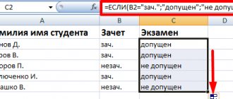
IF. The option is used if the calculation is carried out with the “IF” condition and a large amount of data with different scenarios. Using the function allows you to compare values. If the result is true, the program performs some other action.
MAX and MIN - determine the largest and smallest parameter from the list.

Excel also uses other functions, but they are less in demand.

Terms of use

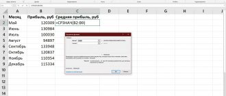
For a better understanding, let's look at how to correctly add a function in Excel. We use the AVERAGE parameter.

The algorithm of actions is as follows:

Click on the cell where you need to set the formula - B11.
Write the equal sign =, and then indicate the name of the desired AVERAGE option.
Specify the range of sections in parentheses (B3:B10).
Click on Enter.

After specifying these parameters, the program summarizes the data in cells B3 to B10, and then calculates their average value.

Using AutoSum

For convenience, almost any option can be inserted using AutoSum. Do the following:

Select and click on the section into which you want to enter the formula (C 11).
In the Editing group in the Home section, find and click on the arrow next to AutoSum.
Select the desired option from the menu that appears, for example, Amount.
The program automatically selects a range of cells to sum, but this data can be set manually by making edits to the formula.

As in the cases discussed above, the result must be checked to avoid errors.

Combination Formulas

An added benefit of Excel is the ability to combine multiple formulas to perform more complex calculations.

Consider a situation where you need to sum three numbers and multiply them by a factor of 1.5 or 1.6, depending on what number you get (more or less than 100).

In this case, the entry has the following form: =IF(SUM(A2:C2)<100,SUM(A2:C2)*1.5,SUM(A2:C2)*1.6).

The above formula uses two options - IF and SUM. In the first case, three results are taken into account - condition, correct or incorrect.

The following conditions apply here:

Excel sums the numbers in cells A2 through C2.
If the resulting number is less than 100, then the parameter is multiplied by 1.5.
If the final figure exceeds 100, then the result is multiplied by 1.6.

Combined Excel formulas are in demand when you need to make different calculations and use more complex formulas.

Useful life hacks: How to install an online consultant on a website, How to work in Trello, How to save a file in pdf format.

Differences in MS Excel versions

Everything described above is suitable for modern programs of 2007, 2010, 2013 and 2016. The old Excel editor is significantly inferior in terms of capabilities, number of functions and tools. If you open the official help from Microsoft, you will see that they additionally indicate in which version of the program this function appeared.

In all other respects, everything looks almost exactly the same. As an example, let's calculate the sum of several cells. To do this you need:

Provide some data for calculation. Click on any cell. Click on the "Fx" icon.

Select the “Mathematical” category. Find the “SUM” function and click on “OK”.

We indicate the data in the required range. In order to display the result, you need to click on “OK”.

You can try to recalculate in any other editor. The process will happen exactly the same.

Types of links and their features

Excel provides relative and absolute references that make life easier for the user and allow you to perform complex calculations. Below we will look at the features of each link.

Relative

Unless you make any changes, all links are relative by default.

For example, when copying the formula =B2+C2 from the second line to the third, the entry will change to =B3+C3. This is useful when you need to copy a calculation across different columns at the same time.

Algorithm of actions when using:

Select and click on the cell (section) where you plan to write the formula (B3).
Enter the data for calculating the parameter of interest - =C3*D3.
Click on enter. The program makes calculations, and the result is shown in the selected section.
Find the auto-fill marker in B3.
Click on it and, holding the left mouse button, move the marker along the desired cells, for example, from B3 to B10.
After releasing the buttons, the formula is copied to all specified sections. At the same time, calculations are performed.

Once again, make sure that the calculations are done correctly.

Absolute links

The tool is used when you need to work with many cells. The point is that when you copy a calculation, the link to the specified section is saved.

Excel uses the dollar symbol ($) to indicate an absolute reference. Depending on the arrangement option, the user's instructions also change.

Let's consider several options:

$A$3 - row/column does not change;
A$3 - the term remains unchanged;
$A3 - the column does not change.

As a rule, the first type of display is used, and the others are almost not used.

For example, let's calculate the tax rate entered in section D1. Since the parameter is identical in all cases, we will introduce the formula $D$1 into the calculation.

For this:

Specify the cell where the formula will be located, for example, C3.
Write the calculation in the form (A3*B3)*$D$1.
Click on the Enter button.
Find the auto-fill marker in C3 (the dot at the bottom right).
Click on it, click on the left mouse button and drag the marker down, grabbing the ranges from C4:C14.
Release the mouse button, after which the formula is copied to the cells with the link. In all cases, automatic calculations are made.

By double-clicking on cells, you can check the correctness of the entered formulas. For all sections, the absolute cell must be identical. When checking, make sure there is a $ symbol. If missed, it will lead to incorrect results.

Now you have at your disposal detailed instructions on how to create a formula in Excel, what functions exist, and how to use them correctly to obtain the correct result. Following these recommendations allows you to quickly understand the calculations and expand the possibilities of using the program.

Sincerely, Alexander Petrenko especially for the project proudalenku.ru

Transcription online

The best CRM systems

Photo stocks

Zoom conference

Makeup artist from scratch

Profession Accountant

VLOOKUP: Search for values

When working with multiple tables, the VLOOKUP function is useful. For example, you have two lists - one contains product numbers, its customers, price and quantity, and the other contains the same product numbers and their description. Such tables can be very large, and item IDs are usually out of order and repeated. To find out which product is hidden under a certain number, use the VLOOKUP function.

In Excel, VLOOKUP was described as follows: it looks for the value in the leftmost column of the table and returns the value of the cell located in the specified column of the same row. That is, she can find information in one table based on similar values from another.

The VLOOKUP arguments are the desired value, the table, the number of the column from which information should be retrieved, and an interval view. The last argument should be set to FALSE if you are looking for an exact value, and TRUE to look for an approximate value.

VLOOKUP is considered a complex function. It can process a large amount of data and find the value you need in a matter of seconds.