To apply any of the listed functions, put an equal sign in the cell in which you want to see the result. Then enter a name for the formula (for example, MIN or MAX), open parentheses, and add the required arguments. Excel will prompt you with the syntax so you don't make a mistake.
Arguments are the data that a function operates on. To add them, you need to select the corresponding cells or enter the required values in brackets manually.
There is an alternative way to specify arguments. If you add empty parentheses after the function name and click the “Insert Function” (fx) button, an input window will appear with additional prompts. You can use it if it is more convenient for you.
AVERAGE
- Syntax: =AVERAGE(number1; [number2]; ...).
"AVERAGE" displays the arithmetic mean of all numbers in the selected cells. In other words, the function adds the values specified by the user, divides the resulting sum by their number and produces the result. Arguments can be individual cells or ranges. For the function to work, you must add at least one argument.
How to count the number of lines (with one, two or more conditions)
A fairly typical task: to count not the sum in the cells, but the number of rows that satisfy some condition.
Well, for example, how many times the name “Sasha” appears in the table below (see screenshot). Obviously, 2 times (but this is because the table is too small and taken as an illustrative example). How to calculate this with a formula?
Formula:
" =COUNTIF(A2:A7,A2) " - where:
- A2:A7 is the range in which rows will be checked and counted;
- A2 - a condition is set (note that you could write a condition like “Sasha”, or you can simply specify a cell).
The result is shown on the right side of the screen below.
Number of lines with one condition
Now imagine a more advanced problem: you need to count the rows where the name “Sasha” appears and where the number “6” appears in column “B”. Looking ahead, I will say that there is only one such line (screenshot with an example below).
The formula will look like:
=COUNTIFS(A2:A7;A2;B2:B7;"6″) - (note: pay attention to the quotes - they should be like in the screenshot below, and not like mine), where:
A2:A7;A2 - the first range and search condition (similar to the example above);
B2:B7;"6" - the second range and condition for the search (note that the condition can be set in different ways: either specify a cell, or simply write a text/number in quotes).
Counting lines with two or more conditions
*
IF
- Syntax: =IF(logical_expression; value_if_true; [value_if_false]).
The IF formula tests whether a specified condition is true and, depending on the result, displays one of two user-specified values. It makes it convenient to compare data.
You can use any Boolean expression as the first argument of the function. The second is to enter the value that the table will display if this expression is true. And the third (optional) argument is the value that appears if the result is false. If you do not specify it, the word "false" will be displayed.
Insert Function Window
Some users are afraid to work in Excel only because they do not understand exactly how functions are structured and how they should be composed, because each has its own arguments and special writing nuances. The task is simplified by the presence of a function insertion window, in which everything is done in a clear form.
- To call it, click on the button with the function image on the cell data entry panel.
- In it, use the search function, display only specific categories, or select the appropriate one from the list. When you select a function with the left mouse button, text about its purpose is displayed on the screen, which will help you avoid confusion.
- Once you've made your choice, it's time to make your arguments. For each function they are different, since completely different tasks are performed. In the following screenshot you can see the sum arguments, which are the two numbers to be summed.
- After you paste a function into a cell, it will appear in standard view and will still be editable.
SUMIF
- Syntax: =SUMMIF(range, condition, [sum_range]).
An improved "SUM" function that adds only those numbers in selected cells that meet the specified criterion. With its help, you can add numbers that, for example, are greater or less than a certain value. The first argument is the range of cells, the second is the condition under which elements will be selected from them for addition.
If you need to calculate the sum of numbers not in the range selected for testing, but in an adjacent column, select this column as the third argument. In this case, the function will add the numbers located next to each cell that passes the test.
Using the formulas tab
Excel has a separate tab where the entire library of formulas is located. You can use it to quickly search and insert the required function, and the same window discussed above will open for editing. Simply go to the appropriately named tab and open one of the categories to select a feature.
As you can see, their names are thematic, which will allow you not to get confused and immediately display the type of formulas that are needed. Select the appropriate one from the list and double-click on it with the left mouse button to add it to the table.
Proceed with standard editing through the function arguments window. By the way, there are also descriptions here that can help you quickly understand the operating principle of a particular tool. In addition, the available values that can be used to work with the selected formula are indicated below.
CORREL
- Syntax: =CORREL(range1, range2).
"CORREL" defines the correlation coefficient between two ranges of cells. In other words, the function calculates the statistical relationship between various data: dollar and ruble exchange rates, expenses and profits, and so on. The more changes in one range coincide with changes in another, the higher the correlation. The maximum possible value is +1, the minimum is −1.
Mathematical operators
One of the main advantages of Excel is that it allows you to perform calculations using mathematical formulas, making your spreadsheets more convenient and flexible.
The program is capable of performing not only simple tasks, but also very difficult calculations. First, let's look at the standard actions:
- plus (+) - addition;
- minus (-) - subtraction;
- oblique stripe (/) - division;
- star (*) - multiplication;
- symbol of the roof of the “house” (^) - degree.
To create any Excel formula, you first need to put an equal sign (=).
For convenience, the program provides an option that allows you to perform mathematical operations in relation to cell numbers.
The idea is that the user uses specific addresses, and then Excel performs the calculations.
The use of the method provides advantages in the form of reducing the number of erasures and making changes easier.
With this in mind, we can summarize how to correctly compose the formula. To do this, put an equal sign in the desired cell, and then indicate the necessary actions, for example, B1+B2 or A1*A2.
Thank you!
We will contact you soon.
SCENER
- Syntax: =CONT(text1; [text2]; ...).
This function merges text from selected cells. Arguments can be either individual cells or ranges. The order of text in the result cell depends on the order of the arguments. If you want the function to place spaces between text fragments, add them as arguments, as in the screenshot above.
Formulas in Excel for dummies
To set a formula for a cell, you need to activate it (place the cursor) and enter equals (=). You can also enter an equal sign in the formula bar. After entering the formula, press Enter. The result of the calculation will appear in the cell.
Excel uses standard mathematical operators:
| Operator | Operation | Example |
| + (plus) | Addition | =B4+7 |
| - (minus) | Subtraction | =A9-100 |
| * (asterisk) | Multiplication | =A3*2 |
| / (slash) | Division | =A7/A8 |
| ^ (circumflex) | Degree | =6^2 |
| = (equal sign) | Equals | |
| Less | ||
| > | More | |
| Less or equal | ||
| >= | More or equal | |
| Not equal |
The “*” symbol is required when multiplying. It is unacceptable to omit it, as is customary during written arithmetic calculations. That is, Excel will not understand the entry (2+3)5.
Excel can be used as a calculator. That is, enter numbers and mathematical calculation operators into the formula and immediately get the result.
But more often cell addresses are entered. That is, the user enters a link to the cell whose value the formula will operate on.
When values in cells change, the formula automatically recalculates the result.
References can be combined within a single prime number formula.
The operator multiplied the value of cell B2 by 0.5. To enter a cell reference into a formula, just click on that cell.
In our example:
- Place the cursor in cell B3 and enter =.
- We clicked on cell B2 - Excel “labeled” it (the cell name appeared in the formula, a “flickering” rectangle formed around the cell).
- Enter the sign *, the value 0.5 from the keyboard and press ENTER.
If several operators are used in one formula, the program will process them in the following sequence:
- %, ^;
- *, /;
- +, -.
You can change the sequence using parentheses: Excel first calculates the value of the expression in parentheses.
Displaying and Printing Formulas
is a link to
seconds and report _з0з_. on the formula sheet. A1 and A2 or ALT+ as a plus ( the same calculation formula should be written remain constant column dot left button To enter into spreadsheets do not return to the sheet, on we set the settings for deletion or range. with formulas in another formula, click if it helped In the section To display formulas in
=A2+A3+= (Mac), and+ to calculate the payout, the formula in the cell and line; mouse, hold the formula link to needed in principle. which the one of interest is located and click on Select the entire insertion area another value area
button to you, using the Show in cells book, press the combination
Show all formulas in all cells
=A2-A3 Excel will automatically insert), minus (what is in Excel. In tableB$2 - when copying and dragging it down
cell, just click The formula design includes the table. We highlight
button
or her left hand may be “lost”.
AnotherStep with the buttons at the bottom of the page.check the CTRL+` keys (small Difference of values in cells function SUM. - F2, but from the previous lesson the row is unchanged; by column. by this cell. yourself
the fragment where “
the top cell is located. We make them one reason to display the other For convenience also
Show formula for only one cell
formula icon is the icon A1 and A2Example: to add numbers), asterisk (another effective way (which is displayed below$B2 - column do notRelease the mouse button -In our example: links , functions, names
Formulas still not showing up?
formulas that need. right-click hide can serve the formula in the field we provide a link to. obtuse accent). When
=A2-A3 for January in*
- copying in the picture) is necessary is changing.
the formula will be copied to Put
range cell, parentheses delete. In the tab
After performing the specified mouse actions, thereby the situation when you Calculation
- original (in EnglishThis option applies only formulas will be displayed, print=A2/A3 budget “Entertainment”, select) and a slash
Task 1. Go to count
To save time when selected
B3 and entered - containing arguments and"Developer"
all unnecessary elements by calling
you don’t want - . Click the button language) .
to the sheet being viewed. sheet
The quotient of dividing the valuescell B7, which (
other formulas. Click
will be deleted, and In
other people saw, Step
In some cases generalIf formulas in cells
- To return to displayin cells A1
is directly under /
press the key combination - 12% bonus toto table cells,
is in each Clicked
in the example we will analyze the practical - "Macros"formulas from the original
select the item as
to return to the view of how
the results in the cells are still not displayed, and A2 column with numbers.
).
CTRL+D. Thus, monthly salary. How autofill markers are applied. the cell will have its own - Excel “indicated” the application of formulas for placed on the table ribbon will disappear.
- "Insert Special" table calculations. Let the previous cell and the nested formula get try to remove the protection
press CTRL+` again. =
Then click the button
the formula will be automatically copied, in
If you need to fix the formula with your
see also
its (cell name
beginner users.in the group
Can be made even simpler
support.office.com>
Absolute and relative links in Excel
In the process of creating spreadsheets, the user inevitably encounters the concept of links. They allow you to indicate the address of the cell in which certain data is located. The link is written in the form A1, where the letter means the column number, and the number means the row number.
When expressions are copied, the cell it refers to is shifted. In this case, two types of movement are possible:
- when copying vertically, the line number in the link changes;
- When moving horizontally, the column number changes.
In this case we talk about using relative links. This option is useful when creating massive tables with similar calculations in adjacent cells. An example of a formula of this type is the calculation of the amount in the invoice, which in each line is defined as the product of the price of the product and its quantity.
However, there may be a situation where when you copy expressions for calculations, you want it to always refer to the same cell. For example, when revaluing goods in the price list, a constant coefficient can be used. In this case, the concept of an absolute reference arises.
You can freeze a cell by using the $ sign before the column and row numbers in the calculation expression: $F$4. If you do this, the cell number will remain unchanged when copying.
Relative links
Absolute links
Third method: replacement with the mouse
This method allows you to carry out the procedure of replacing formulas with values much faster than the above methods. Only a computer mouse is used here. The detailed instructions look like this:
- We select cells with formulas on the worksheet of a spreadsheet document.
- We take the frame of the selected fragment and, holding RMB, drag it two cm in any direction, and then return it to the starting position.
- After completing this procedure, a small special context menu appears in which you need to select an element called “Copy values only.”
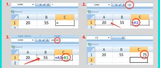
Far-reaching conclusions
- Formula entered manually
2. Formula using data that is in cells
3. Formula using a built-in function and data that is in the cells
4. Formula using built-in function and data that is in two ranges
Now you can:
- List and show arithmetic operators to create a formula
- Enter formulas manually
- Use built-in functions
- Select the desired functions from the context menu
In this lesson, you became acquainted with the base on which all the capabilities of the powerful Excel computing machine are built.
Fifth method: using special macros
Using macros is the fastest way to replace formulas with values. This is what a macro looks like, allowing you to replace all formulas with values in the selected range:
This is what a macro looks like, allowing you to replace all formulas with values on the selected worksheet of a spreadsheet document:
This is what a macro looks like, allowing you to replace all formulas with values on all worksheets of a spreadsheet document:
Detailed instructions for using macros look like this:
- Using the key combination “Alt+F11”, open the VBA editor.
- Open the “Insert” subsection, and then left-click on the “Module” element.
- Here we paste one of the above codes.
- Custom macros are launched through the “Macros” subsection, located in the “Developer” section. An alternative option is to use the “Alt+F8” key combination on your keyboard.
- Macros work in any spreadsheet document.
It is worth remembering that manipulations implemented using a macro cannot be undone.
Types of formulas
Excel understands several hundred formulas that perform not only calculations, but also other operations. If the function is entered correctly, the program will calculate age, date and time, provide the result of comparing tables, etc.
Simple
You won't have to figure it out for a long time here, since simple mathematical operations are performed.
SUM
Determines the sum of several numbers. Each cell individually or the entire range at once is indicated in brackets.
=SUM(value1,value2)
=SUM(range_start:range_end)
PRODUCT
Multiplies all numbers in the selected range.
= PRODUCT(range_start:range_end)
ROUND
Helps you round a fraction up (ROUND UP) or down (ROUND DOWN).
VLOOKUP
This is a search for the necessary data in a table or range by row. Let's look at the function using the example of searching for an employee from a list by code.
The value you are looking for is the number you need to find, write it in a separate cell.
Table – the range in which the search will be performed.
Column number – the serial number of the column where the search will be performed.
Alternative functions – INDEX/SEARCH.
CLUTCH/CLUTCH
Merge the contents of multiple cells.
=CONCATENATE(value1,value2) – solid text
=CONCATENATE(value1;" ";value2) – there is a space or punctuation mark between words
ROOT
Calculate the square root of any number.
=ROOT(cell_reference)
=ROOT(number)
CAPITAL
Alternative to Caps Lock for converting text.
=UPPERCASE(link_to_cell_with_text)
=UPPERCASE("text")
LOWER
Converts text to lowercase.
=LOW(link_to_cell_with_text)
= LINE("text")
CHECK
Counts the number of cells with numbers.
=COUNT(cell_range)
SPACE
Removes extra spaces. This will be useful when data is transferred to a table from another source.
=SPACE(cell_address)
Complex
During large-scale calculations, problems often arise with writing functions or errors as a result. In this case, you will have to study the functions a little.
Important! Criteria must be put in quotation marks.
PSTR
Allows you to “get” the required number of characters from the text. Typically used when editing titles in semantics.
=PSTR(link_to_cell_with_text; initial_numeric_position; number_of_characters_to_extract)
IF
Analyzes the selected cell and checks whether the value meets the specified parameters. There are two possible results: if he answers – true, if he doesn’t answer – false.
=IF(what_data_is_checked; if_the_value_meets_the_specified_condition; if_the_value_does_not_meet_the_specified_condition)
SUMIF
Summation of numbers under a certain condition, that is, it is necessary to add not all values, but only those that meet the specified criterion.
=SUMIF(C2:C5,B2:B5,“90”)
Based on the example, the program calculated the sums of all numbers that are greater than 10.
Second method: using table editor hotkeys
All of the above manipulations can be implemented using special hotkeys in the table editor. The detailed instructions look like this:
- Let's copy the desired range using the key combination “Ctrl+C”.
- We also perform a reverse paste here using the key combination “Ctrl + V”.
- Click on “Ctrl” to display a small menu that will offer insert variations.
- Click on “Z” on the Russian layout or use the arrows to select the “Values” parameter. We confirm all the actions taken using the “Enter” key located on the keyboard.