Correlation analysis is a popular statistical research method that is used to identify the degree of dependence of one indicator on another. Microsoft Excel has a special tool designed to perform this type of analysis. Let's find out how to use this feature.
Purpose of correlation analysis
The dependence is established when the identification of the correlation coefficient begins. This method differs from regression analysis because there is only one indicator, calculated using correlation. The interval varies from +1 to -1. If it is positive, then an increase in the first value contributes to an increase in the 2nd. If it is negative, then an increase in the 1st value contributes to a decrease in the 2nd. The higher the coefficient, the more strongly one value influences the 2nd.
Important! At 0, there is no relationship between the values.
A few important notes
1. The Pearson correlation coefficient is sensitive to outliers. One abnormal value can significantly distort the coefficient. Therefore, outliers should be checked and, if necessary, removed before analysis. Another option is to go to Spearman's rank correlation coefficient. It is also calculated, but not by the initial values, but by their ranks (an example is shown in the video below the article).
2. A synonym for correlation is interconnection or joint variation. Therefore, the presence of a correlation (r ≠ 0) does not yet mean a cause-and-effect relationship between the variables. It is possible that joint variation is due to the influence of a third variable. When variables change together without cause and effect, it is called spurious correlation .
3. The absence of linear correlation (r = 0) does not mean the absence of a relationship. It may be nonlinear. This problem is partially solved by Spearman's rank correlation, which shows the joint increase or decrease in ranks, regardless of the form of the relationship.
The video shows the calculation of the Pearson correlation coefficient with confidence intervals, Spearman's rank correlation coefficient.
Calculation of the correlation coefficient
Let's analyze the calculation using several samples. For example, there is tabular data where spending on advertising promotion and sales volume are described by month in separate columns. Based on the table, we will find out the level of dependence of sales volume on the money spent on advertising promotion.
Method 1: Defining Correlation Using the Function Wizard
CORREL is a function that allows you to implement correlation analysis. The general form is CORREL(array1, array2). Detailed instructions:
- It is necessary to select the cell in which you plan to display the calculation result. Click "Insert Function" located to the left of the text field to enter the formula.
1
- The "Function Wizard" opens. Here you need to find CORREL, click on it, then on “OK”.
2
- An argument window has opened. In the “Array1” line you must enter the coordinates and intervals of the 1st value. In the example under consideration, this is the “Sales value” column. You just need to select all the cells that are in this column. In the “Array2” line, you similarly need to add the coordinates of the second column. In this example, this is the “Advertising costs” column.
3
- After entering all ranges, click on the “OK” button.
The coefficient was displayed in the cell that was indicated at the beginning of our actions. The result obtained is 0.97. This indicator reflects the high dependence of the first value on the second.
4
Method 2: Calculate Correlation Using Analysis Package
There is another method for determining correlation. This uses one of the functions found in the analysis package. Before using it, you need to activate the tool. Detailed instructions:
- Go to the “File” section.
5
- A new window has opened in which you need to click on the “Options” section.
- Click on “Add-ons”.
- Find the “Management” element at the bottom. Here you need to select “Excel Add-ins” from the context menu and click “OK”.
6
- A special add-ons window has opened. Place a checkmark next to the “Analysis Package” element. Click “OK”.
- Activation was successful. Now let's go to "Data". The “Analysis” block appears, in which you need to click “Data Analysis”.
- In the new window that appears, select the “Correlation” element and click on “OK”.
7
- An analysis settings window appeared on the screen. In the “Input interval” line, you must enter the range of absolutely all columns participating in the analysis. In the example under consideration, these are the columns “Sales Value” and “Advertising Costs”. In the output display settings, the “New Worksheet” option is initially set, which means displaying the results on a different sheet. If desired, you can change the location where the result is displayed. After making all the settings, click on “OK”.
8
The final indicators have been displayed. The result is the same as in the first method - 0.97.
Definition and calculation of multiple correlation coefficient in MS Excel
To identify the level of dependence of several quantities, multiple coefficients are used. Subsequently, the results are summarized in a separate table called the correlation matrix.
Detailed Guide:
- In the “Data” section we find the already known “Analysis” block and click “Data Analysis”.
9
- In the window that appears, click on the “Correlation” element and click on “OK”.
- In the “Input interval” line we enter an interval across three or more columns of the source table. The range can be entered manually or simply select it with LMB, and it will automatically appear in the desired line. In “Grouping”, select the appropriate grouping method. The “Output Option” specifies the location where the correlation results will be output. Click “OK”.
10
- Ready! A correlation matrix was constructed.
11
Pair correlation coefficient in Excel
Let's look at how to correctly calculate the pair correlation coefficient in the Excel spreadsheet.
Calculation of pair correlation coefficient in Excel
For example, you have values for x and y.
12
X is the dependent variable, and y is the independent variable. It is necessary to find the direction and strength of the relationship between these indicators. Step-by-step instruction:
- Let's identify the average values using the AVERAGE function.
13
- Let's calculate each x and xaverage, y and average using the “-” operator.
14
- We multiply the calculated differences.
15
- We calculate the sum of the indicators in this column. Numerator – the result found.
16
- Let's calculate the denominators of the difference x and x-average, y and y-average. To do this, let's square it.
17
- Using the AUTOSUM function, we will find the indicators in the resulting columns. We multiply. Using the SQRT function, we square the result.
18
- We calculate the quotient using the values of the denominator and numerator.
19 20
- CORREL is an integrated function that allows you to prevent complex calculations. Go to the “Function Wizard”, select CORREL and indicate the arrays of x and y indicators. We build a graph displaying the obtained values.
21
Pair correlation coefficient matrix in Excel
Let's look at how to calculate the coefficients of paired matrices. For example, there is a matrix of four variables.
22
Step-by-step instruction:
- Go to “Data Analysis”, located in the “Analysis” block of the “Data” tab. In the list that appears, select “Correlation”.
- We set all the necessary settings. “Input interval” is the interval of all four columns. “Output interval” is the place where we want to display the results. Click on the “OK” button.
- A correlation matrix was constructed at the selected location. Each intersection of a row and a column is a correlation coefficient. The number 1 is displayed when the coordinates match.
23
Other features
You can also conduct more complex studies using the CORREL function. An example is pairwise and multiple correlation. Their difference lies in the fact that with multiple correlation there can be two or more independent variables influencing the value, but with pair correlation there can be only one. These tools are used by specialists when analyzing large amounts of data to conduct statistical studies and identify complex dependencies of one value on many others or the absence thereof.
You can also make a graph to clearly show the dependence of one quantity on another. Let's do this for the first example with advertising and sales.
This way of displaying data allows you to quickly assess the impact, and the correlation coefficient shows the strength of the relationship. However, it is not recommended to draw a definitive conclusion based on correlation studies; additional analysis of influencing factors is necessary.
As you can see, Microsoft's Excel editor allows you to conduct statistical studies and identify relationships between data sets using built-in functions. Correlation gives a general idea of how data is related, but more accurate results can only be obtained by using multiple statistical tools.
The CORREL function in Excel is used to calculate the correlation coefficient between two data sets under study and returns the corresponding numeric value.
CORREL function to determine relationship and correlation in Excel
CORREL is a function used to calculate the correlation coefficient between 2 arrays. Let's look at four examples of all the abilities of this function.
Examples of using the CORREL function in Excel
First example. There is a sign that contains information about the average wages of the company’s employees over eleven years and the $ exchange rate. It is necessary to identify the relationship between these two quantities. The plate looks like this:
24
The calculation algorithm looks like this:
25
The displayed value is close to 1. Result:
26
Determining the correlation coefficient of the influence of actions on the result
Second example. Two applicants turned to two different agencies for help to implement an advertising promotion lasting fifteen days. Every day a social survey was conducted to determine the degree of support for each candidate. Any respondent could choose one of two candidates or oppose them all. It is necessary to determine how much each advertising promotion influenced the degree of support for applicants, and which company is more effective.
27
Using the formulas below, we calculate the correlation coefficient:
- =CORREL(A3:A17,B3:B17).
- =CORREL(A3:A17,C3:C17).
Results:
28
From the results obtained, it becomes clear that the degree of support for the 1st applicant increased with each day of the advertising promotion, therefore, the correlation coefficient approaches 1. When the advertisement was launched, the other applicant had a large number of trust, and there was a positive trend for 5 days. Then the degree of trust decreased and by the fifteenth day dropped below the initial indicators. Low scores indicate that promotions had a negative impact on support. Do not forget that other related factors that are not considered in tabular form could also affect the indicators.
Analysis of content popularity by correlation of video views and reposts
Third example. A person uses social networks to promote his own videos on YouTube video hosting. He notes that there is a certain relationship between the number of reposts on social networks and the number of views on the channel. Is it possible to forecast future indicators using spreadsheet tools? It is necessary to identify the reasonableness of using a linear regression equation to predict the number of views of videos depending on the number of reposts. Table with values:
29
Now it is necessary to determine the presence of a relationship between 2 indicators using the formula below:
0.7;IF(CORREL(A3:A8;B3:B8)>0.7;"Strong direct dependence";"Strong inverse dependence");"Weak dependence or its absence")' class='formula'>
If the resulting coefficient is higher than 0.7, then it is more appropriate to use the linear regression function. In the example under consideration we do:
30
Now let's build a graph:
31
We apply this equation to determine the number of views for 200, 500 and 1000 reposts: =9.2937*D4-206.12. We get the following results:
32
The FORECAST function allows you to determine the number of views at a time if, for example, two hundred and fifty reposts were made. We apply: 0.7;PREDICTION(D7;B3:B8;A3:A8);"The quantities are not interrelated")' class='formula'>. We get the following results:
33
Features of using the CORREL function in Excel
This function has the following features:
- Empty cells are not taken into account.
- Cells containing Boolean and Text information are not taken into account.
- Double negation “—” is used to account for logical quantities in the form of numbers.
- The number of cells in the arrays under study must match, otherwise the message #N/A will be displayed.
Examples of using
Let's look at several problems to understand how the statistical function works.
Example 1. A company has a budget for an advertising campaign per month, and there is also a product sales volume; it is necessary to calculate the dependence of these values.
In an arbitrary cell, write a formula with a link to two ranges and get a number.
The result is close to one, which means there is a strong direct relationship between advertising and product sales.
Example 2.
There are furniture sales figures for the quarter, as well as changes in the price of the product over the same period of time.
In this case, the correlation coefficient tends to -1, which indicates a strong inverse relationship. That is, as the price of a product increases, sales fall.
Example 3.
There are expenses for an apartment and food for three months; it is necessary to calculate the dependence of these expense items on each other.
The obtained result indicates a weak connection between these categories.