Author: IsTOPnik
09 September 2022 09:46
Tags: excel pinning useful tips row table photo
1769
12
The Microsoft Excel program is created in such a way that it is convenient not only to enter data into a table and edit it in accordance with a given condition, but also to view large blocks of information.
0
Source:
See all photos in the gallery
The names of columns and rows can be significantly removed from the cells with which the user is working at that moment. And scrolling the page all the time to see the title is uncomfortable. Therefore, the table processor has the ability to pin areas. As a rule, the table has one header. And the lines can be from several tens to several thousand. Working with multi-page table blocks is inconvenient when the column names are not visible. Scrolling all the time to the beginning, then returning to the desired cell is irrational.
Multiple Columns
In the case when the headings are in two or three columns, you need:
- Activate the lowest table cell to the right of the frozen column.
- Select the “Pin…” option and click on the item of the same name.
- This fixes the desired number of columns.
How to Freeze a Column in Excel
Freezing columns in Excel is almost exactly the same as freezing rows. You can freeze just the first column, or freeze multiple columns. Let's move on to examples.
How to Freeze the First Column in Excel
Freezing the first column is just as easy, click “View” -> “Freeze Areas” -> “Freeze First Column”.
Freeze columns and rows in Excel – Freeze the first column in Excel
And still, a darker and thicker border means that the left column is fixed.
Freeze columns and rows in Excel – Freeze first column in Excel
How to Freeze Multiple Columns in Excel
If you want to freeze 2 columns or more on a sheet, then proceed as follows:
- Select the column to the right of the last column you want to freeze. For example, if you want to freeze 3 columns in Excel (A, B, C), select the entire column D or cell D1
Note that anchored columns always start from the leftmost column (A). That is, it is impossible to anchor one or more columns somewhere in the middle of the sheet.
Freeze Columns and Rows in Excel – Highlight the column you want to freeze the columns before
- And now follow the already familiar path, that is, in the “View” tab -> “Freeze areas” -> and again “Freeze areas”.
Freeze Columns and Rows in Excel – Freeze Three Columns in Excel
Make sure that all the columns you want to freeze are visible when you freeze them. If some of the columns are out of view (i.e. hidden), you won't see them later.
How to freeze a row and column in Excel
Do you want to freeze a column and a row at the same time ? No problem, you can do this, provided you always start with the top row and first column .
To freeze multiple rows and columns at once, select the cell below the last row and to the right of the last column you want to freeze.
For example, to freeze the first column and first row , select cell B2, go to the View tab, and click Freeze Panes under Freeze Panes.
Freeze Columns and Rows in Excel – Freeze Rows and Columns in Excel
Now both the row and the column are fixed in the Excel sheet .
Freeze Columns and Rows in Excel – Freeze First Column and First Row
In the same way, you can dock as many panels in Excel as you want. For example, to freeze the first 2 rows and 2 columns, you select cell C3; to freeze 3 rows and 3 columns, select cell D4, etc. Naturally, the number of frozen rows and columns does not have to be the same. For example, to freeze 2 rows and 3 columns, you select cell D3.
Fixing a cell in a formula
You can also fix the formula in Excel. It is created indicating the addresses of the cells, the data from which is involved in the calculations. If you copy such formulas in the appropriate directions, they will perform the calculation in the cell.
First, an absolute reference to the cell in the first formula is created. This will fix it and will work when stretched. You need to enter the formulas, click on the second cell with the mouse and press F4. The result is dollar signs before the letter and after the second part of the formula. You must press Enter and copy. Calculations should take place automatically.
If you press F4 each time, you will get different results:
- Fixing the address.
- Assigning a line number. When copied, the column will change.
- Fixing the column name. When copying, only the numbers will change.
- Removing fastening.
The user can freeze a row and a column separately or together in Excel. It is also possible to remove the settings.
How to remove fixation
You will need to unfasten a commit if you make a mistake or erroneous action in the previous lists; otherwise, the procedure is similar:
- go to the “View” menu item;
- select the action “Freeze areas”;
- Click on the first of all the proposed menu options - “Unlock areas”.
Now there are no fixed stripes left in any direction. The difficulty of the work lies in the order of actions and care.
Basic Concepts
The Ribbon is the area at the top of the Excel window containing tabs.
Tabs are tools that summarize groups of specific actions into categories.
What is the pinning function for? By separating the main part from the rest of the text, you will always see the “header” of the table and understand which row you are viewing. This will prevent errors in your work. Cells in a pinned area do not change their position no matter what actions you perform in the program.
Microsoft Excel: Freeze a row on a sheet
a very useful feature, at the same time the entire area is frozen, which scrolling is quite inconvenient.and selectFreeze the first columnAfter clicking all are fixedTo freeze several columns, Excel versions 2007 the “Freeze top function works in we select this list that appears After this, even in this, as if In our example scroll through the worksheet of areas and division since, applying it turns out the entire area will be located above Excel developers as
Pin areasOn a tab
Lock the top row
area of the worksheet you need to select the cell and 2010. In the line.” moment. And all the position “Unpin in case you are far away from we scrolled to Excel, but are pinned
windows. the function of pinning areas, to the left of it. and to the left of this time we took care of. The view is unlocked.
Below the top line there is time to scroll the page, areas.”
In order to unpin the cells will be pinned. for the convenience of users by introducingOn thetab, click theNote button. Button “Unlock the table to the RIGHT of (2003 and 2000) boundary line. Now to see the title, Following this, the top very bottom of the range down, the top line To unfreeze the lines of the field of view in to constantly see certain ease of work in the pinned areas, not
Unbinding the top row
After this, click on in this program View Freeze Areas of Excel 2003 fixed column. And the “Freeze Areas” tool
It’s uncomfortable when scrolling vertically. Therefore, the line will be detached, data with a large
will always remain or columns, click the top of the sheet. areas in the Microsoft Excel work program, you need to select cells. the “Freeze areas” button, the ability to freeze areas. select items
and select item
lumpics.ru>