Microsoft Excel is convenient for creating tables and making calculations. A workspace is a set of cells that can be filled with data. Subsequently – format, use for building graphs, charts, summary reports.
Working in Excel with tables for novice users may seem difficult at first glance. It differs significantly from the principles of creating tables in Word. But we'll start small: by creating and formatting a table. And at the end of the article, you will already understand that you cannot imagine a better tool for creating tables than Excel.
Formula Basics
Because Excel's main goal is to simplify calculations, it provides powerful mathematical tools.
Most of them are of interest only to professionals in a particular industry, but some are also useful to ordinary users. Any formula begins with an equal sign. For simple calculations, you can use classic mathematical operators grouped on the keyboard.
Place the “=” sign in a cell or line for formulas “fx”
Here are examples of such formulas:
- addition – “=A1+A2”;
- subtraction – “=A2-A1”;
- multiplication – “=A2*A1”;
- division – “=A2/A1”;
- raising to a power (square) – “=A1^2”;
- compound expression – “=((A1+A2)^3-(A3+A4)^2)/2”.
The cell address in the formula does not have to be entered manually; you just need to left-click on the desired cell. Knowing this, you can easily and quickly enter any simple expression directly into a cell or into the “fx” line, using only mathematical signs and numbers. More complex functions are specified using literal operator commands.
Using the left mouse button, select the cells with values between them and put the desired mathematical sign from the keyboard
Pivot tables generator and data report designer
Pivot tables are indispensable when creating and designing reports in Excel.
Task 7: Generate a report - how many types of “Personal Care” product range were sold in Russia and what was the average monthly margin in 2006?
Excel solution for all problems #7 using one pivot table.
It would take several books to describe all the capabilities of pivot tables. But you can understand their operating principle even with one small example.
You can download all examples and view them in detail in one file on different sheets. The Excel program is also actively used for maintaining a family budget, drawing up estimates, planning repairs and many other life tasks that a modern person sets for himself every day. The skills in this program help you quickly, easily and efficiently cope with a large number of similar tasks.
All these skills will make you a master of success, because mastery is achieving higher results with less effort.
Initial stage of work
To learn how to work in Excel on your own, start with the simplest steps. The information below will help you with this.
The initial and simplest stage of work involves editing cells. This process means in Excel entering data into a cell area or performing other manipulations with the contents in it.
To get started, create an Excel document, give it a name and open it. Having selected the required cell with one click of the left mouse button, enter text or numeric values in its field. This process will be reflected in two places at once: in the cell itself and in the formula bar, which is marked fx and is located immediately above the table.
The entered information will only be saved after pressing the Enter key.
Working with cell data in Excel is easy:
- Deleting an incorrectly entered character is done using the BackSpace key (if the data has not yet been saved). After pressing the Enter button, you can edit the information only after reactivating the cell. In this case, the data previously entered into this field will be deleted.
- If you want to partially change the text or numeric values, double-click the field to activate it. As a result, a cursor will appear. Install it in the right place and delete the incorrect part of the data using the BackSpace button (deleting a character to the left of the cursor) or Delete (deleting a character to the right of the cursor).
How to compare data in two tables
Users often need to compare two tables in Excel to see if they match. Examples from “life”: compare the prices of goods in different deliveries, compare balances (accounting reports) for several months, the performance of pupils (students) of different classes, in different quarters, etc.
To compare 2 tables in Excel, you can use the COUNTIF operator. Let's look at how to use the function.
For example, let's take two tables with the technical characteristics of different food processors. We decided to highlight the differences with color. Conditional formatting solves this problem in Excel.
Initial data (tables we will work with):
Select the first table. Conditional formatting - create a rule - use a formula to determine which cells to format:
In the formula bar we write: =COUNTIF (compared range; first cell of the first table) = 0. The range being compared is the second table.
To enter a range into a formula, simply select its first cell and the last one. "=0" means a command to search for exact (not approximate) values.
We select the format and set how the cells will change if the formula is followed. It's better to fill it with color.
Select the second table. Conditional formatting – create a rule – use a formula. We use the same operator (COUNTIF).
Here, instead of the first and last cells of the range, we inserted the column name that we assigned to it in advance. You can fill out the formula in any of the following ways. But with a name it’s easier.
Comparing two ranges for differences and similarities
Sometimes when working in Excel, you need to compare two lists and quickly find the elements that are the same or different. Here is the fastest and most visual way to do this:
- Select both columns to compare (hold down the Ctrl key).
- Select on the Home tab → Conditional Formatting → Highlight Cell Rules → Duplicate Values.
- Select the Unique option from the drop-down list.
How to use simple formulas in a program
To understand how the formulas work in the program, you can first look at some simple examples. One such example is the sum of two values.
To do this, you need to enter one number in one cell, and another in the second.
For example, In Cell A1 there is the number 5, and in Cell B1 there is 3. In order for the total value to appear in Cell A3, you must enter the formula:
=SUM(A1;B1).
Calculating the sum of two numbers
Every person can determine the sum of the numbers 5 and 3, but you do not need to enter the number in cell C1 yourself, since this is the intent of calculating the formulas.
After entering, the total appears automatically.
Moreover, if you select cell C1, then the calculation formula is visible in the top line.
If one of the values is changed, recalculation occurs automatically.
For example, when replacing the number 5 in cell B1 with the number 8, there is no need to change the formula; the program itself will calculate the final value.
In this example, calculating totals looks very simple, but it is much more difficult to find the sum of fractional or large numbers.
Sum of fractions
In Excel, you can perform any arithmetic operations: subtraction “-”, division “/”, multiplication “*” or addition “+”.
The formula specifies the type of operation, the coordinates of the cells with the original values, and the calculation function.
Any formula must begin with a “=” sign.
If you do not put “equals” at the beginning, the program will not be able to produce the required value, since the data was entered incorrectly.
Differences between Microsoft product versions
It is worth understanding that Excel 2003 has long been obsolete. There are a huge number of modern features and capabilities missing. In addition, the appearance of various objects (graphs, diagrams, etc.) is much inferior to modern requirements.
Example Excel 2003 workspace.
In modern 2007, 2010, 2013, and even more so 2016 versions, everything is much “cooler”.
Many menu items are located in different sections. Some of them have completely changed their name. For example, the “Formulas” we are familiar with back in 2003 were called “Functions”. And they didn't take up much space.
Now there is a whole tab dedicated to them.
Limitations and capabilities of different versions
On the official Microsoft website you can find online help that provides all the technical characteristics of the books being created.
An example of the most basic parameters.
This list is quite long. Therefore, it is worth following the link and familiarizing yourself with the rest.
Please note that the 2003 version is not even considered since it is no longer supported.
But in some budget organizations this office suite is still used to this day.
How to create a table
Knowledge of how to work in Excel is unlikely to be useful to a user if he does not know how to create a table. The easiest way is to highlight a certain range and mark the boundaries with black lines by clicking on the corresponding icon at the top of the page. But often a non-standard table for forms or documents is required.
First of all, you need to decide what the table should look like in order to set the width and length of the cells. Having selected the range, you need to go to the “Format Cells” menu and select “Alignment”. The “Merge Cells” option will help remove unnecessary borders. Then you need to go to the “Borders” menu and set the required parameters.
Using the Format Cells menu, you can create different table options by adding or removing columns and rows, and changing borders.
Knowing how to work in an Excel table, the user will be able to create headings. To do this, in the “Table Formatting” window, you need to check the box next to the “Table with headers” item.
To add elements to a table, you must use the Design tab. There you can select the required parameters.
Creating tables
You can store any data in Excel tables. Using the quick setup and formatting function, it is very easy to organize a personal budget control system, a list of expenses, digital data for reporting, etc. in the editor.
Tables in Excel have an advantage over a similar option in Word and other office programs. Here you have the opportunity to create a table of any size. The data is easy to fill out. There is a function panel for editing content. In addition, the finished table can be integrated into a docx file using the usual copy-paste function.
To create a table, follow the instructions:
- Open the Insert tab. On the left side of the options panel, select Table. If you need to consolidate any data, select the “Pivot Table” item;
- Using the mouse, select the space on the sheet that will be allocated for the table. And also you can enter the location of the data in the element creation window;
- Click OK to confirm the action.
Rice. 8 – creating a standard table
To format the appearance of the resulting sign, open the contents of the designer and in the “Style” field, click on the template you like. If desired, you can create your own view with a different color scheme and cell highlighting.
Rice. 9 – table formatting
Result of filling the table with data:
Rice. 10 – completed table
How to Create a Table in Excel for Dummies
Working with tables in Excel for dummies is not rushed. You can create a table in different ways, and for specific purposes, each method has its own advantages. Therefore, first let’s visually assess the situation.
Take a close look at the spreadsheet worksheet:
This is a set of cells in columns and rows. Essentially a table. Columns are indicated in Latin letters. Lines are numbers. If we print this sheet, we will get a blank page. Without any boundaries.
First let's learn how to work with cells, rows and columns.
How to select a column and row
To select the entire column, click on its name (Latin letter) with the left mouse button.
To select a line, use the line name (by number).
To select several columns or rows, left-click on the name, hold and drag.
To select a column using hot keys, place the cursor in any cell of the desired column - press Ctrl + spacebar. To select a line – Shift + spacebar.
How to change cell borders
If the information does not fit when filling out the table, you need to change the cell borders:
- Move manually by clicking the cell border with the left mouse button.
- When a long word is written in a cell, double-click on the column/row border. The program will automatically expand the boundaries.
- If you need to maintain the column width, but increase the row height, use the “Wrap Text” button on the toolbar.
To change the width of columns and height of rows at once in a certain range, select an area, increase 1 column/row (move manually) - the size of all selected columns and rows will automatically change.
Note. To return to the previous size, you can click the “Cancel” button or the hotkey combination CTRL+Z. But it works when you do it right away. Later it won't help.
To return the lines to their original boundaries, open the tool menu: “Home” - “Format” and select “Auto-fit line height”
This method is not relevant for columns. Click "Format" - "Default Width". Let's remember this number. Select any cell in the column whose borders need to be “returned”. Again “Format” - “Column Width” - enter the indicator specified by the program (usually 8.43 - the number of characters in the Calibri font with a size of 11 points). OK.
How to insert a column or row
Select the column/row to the right/below the place where you want to insert the new range. That is, the column will appear to the left of the selected cell. And the line is higher.
Right-click and select “Insert” from the drop-down menu (or press the hotkey combination CTRL+SHIFT+”=”).
Oh and click OK.
Advice. To quickly insert a column, select the column in the desired location and press CTRL+SHIFT+"=".
All these skills will come in handy when creating a table in Excel. We will have to expand the boundaries, add rows/columns as we work.
Step-by-step creation of a table with formulas
- We manually fill in the header - the names of the columns. We enter the data and fill out the lines. We immediately put the acquired knowledge into practice - we expand the boundaries of the columns, “select” the height for the rows.
- To fill out the “Cost” column, place the cursor in the first cell. We write “=”. Thus, we signal to Excel: there will be a formula here. Select cell B2 (with the first price). Enter the multiplication sign (*). Select cell C2 (with quantity). Press ENTER.
- When we move the cursor to a cell with a formula, a cross will form in the lower right corner. It points to the autocomplete marker. We grab it with the left mouse button and drag it to the end of the column. The formula will be copied to all cells.
- Let's mark the boundaries of our table. Select the range with the data. Click the button: “Home” - “Borders” (on the main page in the “Font” menu). And select “All borders”.
Column and row borders will now be visible when printing.
Using the Font menu, you can format Excel table data as you would in Word.
Change, for example, the font size, make the header “bold”. You can center the text, assign hyphens, etc.
Displaying data from an Excel spreadsheet on a map
In Excel, you can quickly display your geodata, such as sales by city, on an interactive map. To do this, you need to go to the “App Store” (Office Store) on the “Insert” tab and install the “Bing Maps” plugin from there. This can also be done via a direct link from the site by clicking the Get It Now button.
After adding a module, you can select it from the My Apps drop-down list on the Insert tab and place it on your worksheet. All you have to do is select your data cells and click on the Show Locations button in the map module to see our data on it. If desired, in the plugin settings you can select the type of chart and colors to display.
Creation of tables, types and features of the data contained in them
The workspace of a Microsoft Excel sheet is divided by conditionally invisible borders into columns and rows, the sizes of which can be adjusted by “dragging” the slider placed on the border. To quickly merge cells, use the corresponding icon in the “Alignment” block of the “Home” tab.
In the “Home” tab, in the “Alignment” block, there are tools for merging and aligning cells
The columns are designated by letters of the Latin alphabet (A, B, C,... AA, AB, AC...), the rows are numbered. Thus, each cell has its own unique address. Here is an example of highlighting cell C7.
The selected cell has its own unique address C7, which consists of a column letter and a row number
A cell can contain a numeric value, formatted text, symbols, formulas, and other elements. By default, numbers are located on the right side of the cell, text is on the left. When you select a cell with a formula, the latter is displayed in the “fx” line.
Cells can contain numeric values, text, symbols, formulas, and other elements
Using the tools on the Home tab, you can format cells and the table itself, set the desired text sizes and parameters, highlight borders, apply cell fill, and also perform a number of more complex operations.
Select the cells, in the “Home” tab, click on the appropriate formatting tool icons
By right-clicking on a selected cell or block of cells, you can open a context menu. It consists of a top block that duplicates the main functions of the Home tab and a bottom block that concentrates the operations of copying and pasting text, filtering and sorting values, as well as some other functions.
By right-clicking on a selected cell or block of cells, call up the context menu to format them
By selecting the “Cell Format” item in the context menu, you will get advanced formatting options for the selected data array.
Click on “Format Cells”
Using the window that opens, you can configure as precisely as possible all the features of presenting information in cells and table blocks.
Format Cells window with tools to fine-tune and format cells
In addition, you can apply ready-made styles grouped in the “Conditional Formatting”, “Format as Table” and “Cell Styles” items.
In the “Styles” group in the “Home” tab, you can select a ready-made style
The context menus of these items contain templates with contrasting, gradient and many other formatting schemes, with which you can quickly bring the table block into the desired form.
Ready-made templates for the “Format as table” item
In addition to the already discussed “Font”, “Alignment” and “Styles” groups, the “Home” tab contains several less popular, but still necessary in some cases, elements. On it you can find:
- “Clipboard” – icons for copying, cutting and pasting information (they are duplicated by the key combinations “Ctrl+C”, “Ctrl+X” and “Ctrl+V”, respectively);
- “Number” – provides quick switching between text, numeric, percentage and other information display formats, as well as simple data formalization operations, for example, changing the number of decimal places in fractional numbers;
- “Cells” - contains commands for adding and deleting rows, columns, arrays, as well as simple functions for formatting their size and visibility;
- “Editing” – simplifies searching, sorting and filtering data, includes several quick formulas, performs autofill and autoclear commands.
The arrows in the lower right corner of most Home tab blocks bring up expanded context menus or pop-ups that provide more precise and more complete lists of possible commands.
A small down arrow next to the group name brings up a dialog box with more advanced information or functions
The face of the program
Before you figure out how to work in Excel, it’s worth studying the interface. The tools are located at the top and bottom of the window, and the rest of the area is occupied by rectangles, which are cells. The peculiarity of spreadsheets is that actions can be performed in some cells, and the result can be displayed in others.
Each table has columns that are designated by letters of the English alphabet. Lines are numbered on the left. Thus, any cell has its own coordinates. You can enter both data and formulas in each cell. Before entering the latter, you must put the “=” symbol.
Introduction to Spreadsheets
Each cell in a spreadsheet is called a cell. Which has its own designation - a name. As a rule, the cell name is specified by the column name and row number at the intersection of which it is located. For example, G5,E8.
The main types of data for processing in spreadsheets that can be processed and written into table cells are numbers, text and formulas.
Numbers can take integer and fractional values.
Any sequence of characters, including numbers, is considered text
A formula is a record starting with the “=” (equal) sign, containing cell addresses, arithmetic operations signs, numbers and functions.
A document created in Excel is called a workbook and can contain several sheets, the labels of which are located at the bottom of the window. When saving a workbook in Excel, all sheets will also be saved in a single file.
Adding graphs to charts
To build a chart or graph, you need to have a ready-made plate, because graphical data will be based precisely on information taken from individual rows or cells.
To create a chart/graph you need:
- Select the table completely. If you need to create a graphic element only to display the data of certain cells, select only them;
- Open the insert tab;
- In the recommended charts field, select the icon that you think will best visually describe the tabular information. In our case, this is a three-dimensional pie chart. Move the pointer to the icon and select the appearance of the element;
Rice. 11 – selecting the type of diagram to use
Click on the required form. The already completed diagram will automatically appear on the sheet:
Rice. 12 – result of adding a diagram
If you need to change the appearance of the resulting visualization, simply double-click on it. There will be an automatic redirection to the designer window. With its help, you can apply a different style to the chart, change its type, color scheme, data display format, add new elements and customize them.
In a similar way, you can create scatter plots, line diagrams, and table element dependency diagrams. All received graphic elements can also be added to Word text documents.
The Excel spreadsheet editor has many other functions, however, the techniques described in this article will be sufficient for initial work. In the process of creating a document, many users independently master more advanced options. This happens thanks to the convenient and understandable interface of the latest versions of the program.
Thematic videos:
Microsoft Excel for Beginners #1
Microsoft Excel for Beginners #2
Sparklines
Sparklines are miniature diagrams drawn directly in cells that visually display the dynamics of our data. To create them, click the Line or Columns button in the Sparklines group on the Insert tab. In the window that opens, specify the range with the original numerical data and the cells where you want to display sparklines.
After clicking the “OK” button, Microsoft Excel will create them in the specified cells. On the “Design” tab that appears, you can further configure their color, type, enable the display of minimum and maximum values, and so on.
HOW TO DEnote A CONSTANT CELL IN AN EXCEL FORMULA
There are two types of cell references: relative and absolute. When copying a formula, these links behave differently: relative ones change, absolute ones remain constant.
The program considers all cell references to be relative unless the user specifies another condition. Using relative references, you can multiply the same formula across multiple rows or columns.
- Let's manually fill in the first columns of the training table. We have this option:
2. Let us remember from mathematics: to find the cost of several units of goods, you need to multiply the price for 1 unit by the quantity. To calculate the cost, enter the formula in cell D2: = unit price * quantity. Formula constants are references to cells with corresponding values.
3. Press ENTER - the program displays the multiplication value. The same manipulations must be performed for all cells. How to set a formula for a column in Excel: copy the formula from the first cell to other rows. Relative links are helpful.
Find the autofill marker in the lower right corner of the first cell of the column. Click on this point with the left mouse button, hold it and “drag” it down the column.
Release the mouse button - the formula will be copied to the selected cells with relative links. That is, each cell will have its own formula with its own arguments.
The references in the cell are related to the row.
A formula with an absolute reference refers to the same cell. That is, when autofilling or copying, the constant remains unchanged (or constant).
To point Excel to an absolute reference, the user needs to include a dollar sign ($). The easiest way to do this is with the F4 key.
- Let's create the line "Total". Let's find the total cost of all goods. Select the numeric values of the “Cost” column plus one more cell. This is the range D2:D9
2. Let's use the autocomplete function. The button is located on the “Home” tab in the “Editing” tool group.
3. After clicking on the “Sum” icon (or the ALT+“=” key combination), the selected numbers are added together and the result is displayed in an empty cell.
Let's create another column where we calculate the share of each product in the total cost. To do this you need:
- Divide the cost of one product by the cost of all products and multiply the result by 100. The reference to the cell with the total cost value must be absolute so that it remains unchanged when copied.
2. To get percentages in Excel, it is not necessary to multiply the quotient by 100. Select the cell with the result and click “Percentage Format”. Or press the hotkey combination: CTRL+SHIFT+5
3. Copy the formula to the entire column: only the first value in the formula (relative reference) changes. The second (absolute reference) remains the same. Let's check the correctness of the calculations and find the result. 100%. Everything is correct.
The following absolute reference formats are used when creating formulas:
- $B$2 – when copying, the column and row remain constant;
- B$2 – the string remains unchanged when copied;
- $B2 – column does not change.
Finding and using the right expressions
Several quick commands for automatic data calculation are available in the “Editing” item of the “Home” tab. Suppose we have a series of numbers (sample) for which we need to determine the total and the average. Let's do the following:
Step 1. Select the entire sample array and click on the arrow next to the “Sigma” sign (circled in red).
Select the entire sample array and click on the arrow next to the “Sigma” sign
Step 2. In the context menu that opens, select the “Amount” item. The result of the calculation will appear in the cell located under the array (in our case, cell “A11”).
In the context menu that opens, select “Amount”
Step 3. Now the formula bar displays the expression selected by the system for calculation. The same operator can be entered manually or found in the general catalog.
The formula bar displays the expression selected by the system for calculation
Step 4. Select the sample again and click on the “Sigma” sign, but this time select the “Average” item. The arithmetic mean of the sample will appear in the first free cell of the column, located under the result of the previous calculation.
Select the sample, click on the “Sigma” sign and select “Average”
Step 5. Usually, only simple calculations are performed from the “Home” tab, but in the context menu you can find any necessary formula. To do this, select the “Other functions” item.
Click on the “Sigma” sign and select “Other functions”
Step 6. In the “Function Wizard” window that opens, set the category of the formula (for example, “Mathematical”) and select the desired expression.
In the “Function Wizard” window that opens, set the formula category and select the desired expression
Step 7. Read a brief explanation of the mechanism of action of the formula to make sure that you have chosen the right expression. Then clicks "OK".
We read a brief explanation of the mechanism of action of the formula, click “OK”
Step 8. The selected operator will appear in the formula line, after which you will only have to select a cell or array with data for calculation.
On a note! In addition to the “Editing” item, you can select an operator directly on the “Formulas” tab.
You can select the desired operator directly on the “Formulas” tab
Here the expressions are also collected into a number of categories, each of which contains formulas of a given order. After selecting a specific formula, you will be prompted to enter arguments. You can set values using the keyboard, or you can select a cell or data array with the mouse.
Reference! Over time, the basic operators will remain in memory, and to use them it will be enough to put an equal sign, hold down “Caps Lock” and enter the abbreviated name of the function.
Another important nuance that can make working with formulas much easier is auto-completion. This is the application of one formula to different arguments with automatic substitution of the latter.
The figure below shows a matrix of numerical values and several indicators are calculated for the first row:
- sum of values: =SUM(A3:E3);
- product of values: =PRODUCT(A3:E3);
- square root of a fraction of a sum in a product: =ROOT(G3/F3).
Table with calculations of several indicators for the first line
Let's assume that a similar calculation needs to be performed for the remaining series. To do this, pull the cells with formulas sequentially by the lower right corner down to the end of the numerical values.
Select the cells with formulas and drag the lower right corner down to the end of the numeric values
Please note that the cursor has turned into a “plus”, and the cells behind it are highlighted with a dotted frame. By releasing the mouse button, we get the indicator values calculated by row. Autocomplete can be applied to a single row or column, or to large data sets.
Excel interface
The Excel 2013 application interface is very similar to the Excel 2010 interface. If you have already worked with Excel 2010, then mastering Excel 2013 will not be difficult. If you are new to Excel or have worked primarily with earlier versions, mastering the Excel 2013 interface will take some time.
The first time you open Excel, the Start screen appears. Here you can create a new workbook, select a template, or open one of the latest workbooks.
- Find and open Blank Workbook on the Start screen to see the MS Excel interface.
- The interface of Microsoft Excel 2013 will open in front of you.
Ribbon
The Ribbon is the main working element of the MS Excel interface and contains all the commands necessary to perform the most common tasks. The ribbon consists of tabs, each of which contains several groups of commands.
Quick Access Toolbar
The Quick Access Toolbar lets you access basic commands no matter which Ribbon tab is currently selected. By default, it includes commands such as Save, Cancel, and Redo. You can always add any other commands you want.
Team Group
Each group contains a block of different commands. To apply a command, click on the required shortcut. Some groups contain an arrow in the lower right corner, which you can click to see even more commands.
Field Name
The Name field displays the address or name of the selected cell. If you look closely at the image below, you will notice that cell B4 is the intersection of column B and row 4.
Formula Bar
The formula bar allows you to enter data, formulas, and functions that will also appear in the selected cell. For example, if you select cell C1 and enter the number 1984 in the formula bar, then exactly the same value will appear in the cell itself.
Column
A column is a group of cells that is arranged vertically. In Excel, columns are usually denoted using Latin letters. In the figure below, column H is highlighted.
Cell
Each rectangle in an Excel workbook is usually called a cell. A cell is the intersection of a row and a column. To select a cell, simply click on it. The dark outline around the currently active cell is called the table cursor. In the image below, cell B3 is selected.
Line
A row is a group of cells that is arranged horizontally. Rows in Excel are usually denoted by numbers. In the figure below, line 10 is highlighted.
Worksheet
Excel files are called Workbooks. Each workbook consists of one or more sheets (tabs at the bottom of the screen). They are also called spreadsheets. By default, an Excel workbook contains only one sheet. Sheets can be added, deleted and renamed. You can move from one sheet to another simply by clicking on its name.
Sheet View Modes
There are three main sheet viewing modes. To select the desired mode, simply click the appropriate tab.
- Normal mode is selected by default and shows you an unlimited number of cells and columns.
- Page Layout – Divides the sheet into pages. Allows you to view the document as it will be printed. Also in this mode it becomes possible to configure headers and footers.
- Page mode – allows you to view and adjust page breaks before printing a document. In this mode, only the area of the sheet filled with data is displayed.
Scale
Touch, hold and move the slider to adjust the zoom. The numbers to the right of the slider display the scale value in percentage.
Section 6: Additional
- Interface setup
- How to customize the Ribbon in Excel 2013
- Touch mode for the Ribbon in Excel 2013
- Link styles in Microsoft Excel
Want to learn even more about Excel? Especially for you, we have prepared two simple and useful tutorials: 300 Excel examples and 30 Excel functions in 30 days.
The lesson was prepared for you by the site team Author: Anton Andronov Rules for reprinting Even more lessons on Microsoft Excel
Rate the quality of the article. Your opinion is important to us:
