VLOOKUP function in Excel - quick data transfer
The simplest use of the VLOOKUP function is to quickly transfer data from one table to another.
For example, you have a large price list for 500 items and a request from a buyer, say, for 50 items (in reality, both the price and request can be much higher, but the principle does not change).
You need to quickly find prices for these 50 items. Of course, you can separately search for each item in a large price list and spend 30–60 minutes on it, or you can do it in less than a minute using the VLOOKUP function.
So, we have 500 items in the price list. Positions are designated as follows: letters indicate the type of position, and numbers indicate modification.
For example, “Chair_1” and “Chair_21” are two completely different chairs.
The prices in the price list are given as an example and are unlikely to be related to real prices.
Let's define the task.
YkeA LLC received a request from Petrovich.
Petrovich is a simple person, he likes to do everything quickly, but not very clearly. Therefore, his requests are characterized by a special confusion in positions.
However, this does not frighten us, firstly, we have CDF, and secondly, we have not seen anything like this.
Petrovich demands that we put prices in his request very quickly. He intends to wait a maximum of 5 minutes. After all, other suppliers have already flooded him with offers.
We don’t want to lose such a client and we almost instantly open the price list:
It turns out that we should have two files open (two books in Excel). Request from Petrovich and Price.
This is exactly what is needed, all that remains is to transfer the prices from the price list to the request.
To do this, let’s go to the query table and in the first cell of the “Prices” column (D4) enter “=req” and double-click on the function icon:
Immediately after this, in the formula line you need to place the cursor inside the VLOOKUP inscription and press Fx, a window with the arguments of the VLOOKUP function will appear in front of you:
In the function arguments, you tell Excel what and where to look:
The value you are looking for is the value (in this case, the name) whose price you want to find in the price list. Accordingly, click on the first cell of the “Name” column.
Next, go straight to “Price”:
Now fill in the following fields in the function arguments:
Table - select the columns that contain the desired items and prices, so that the items are the leftmost column.
This is how the VLOOKUP function works - it looks for the required values in the leftmost column (for VLOOKUP this is column No. 1). When VLOOKUP finds the desired value, it begins to look to the right, in the column that you specified in the “Column number”.
There you must specify the column containing the data required for transfer. In our case, these are prices and in our case this is column number two, relative to the table that you specified in the arguments.
Interval viewing - set to 0. Zero indicates an exact match.
After filling in the function arguments, click “Ok” and if everything is done correctly, the price will appear in the “Price” column (file “Request from Petrovich”).
You need to stretch the prices for the remaining cells:
Colleagues, that’s all, you have mastered the VLOOKUP function.
Very important note!
Please note that we were now working in two different files (books).
When work is done in two different books, Excel automatically anchors the table in the VLOOKUP function:
He does this using the $ sign, which he places in front of the columns and rows of the table.
This allows the formula to not move when you pull it down. This is very important when you work within one sheet or one workbook (in this case, Excel does not automatically freeze cells).
Let's see what happens if we stretch the formula “without fixing”:
Please note that for the first cell everything is in order and the range B3:C502 exactly corresponds to the table that we selected for data search, however (without pinning) this will not always be the case; as the VLOOKUP formula is “stretched” down, the table will also shift until one day we see this strange inscription #N/A:
#N/A means that the VLOOKUP function could not find the price of Chair_13 in the price list, and this is not surprising, because the table range in the VLOOKUP formula went below this value:
Therefore, if you don’t want people to leave you, fix the range.
Very important note #2
As you noticed, formulas refer to specific cells, in other words, there is a connection between the formulas and the source data. Once you change the source data, the values in the formulas will immediately change.
This is felt especially acutely in the VPR. If you suddenly forget and add an extra column in the “wrong place” in the original table, then the VLOOKUP formula will produce completely unexpected values.
Therefore, if you do not need a relationship between tables, I recommend turning formulas into data.
To do this, you need to select the column with formulas, press Ctrl+C and in the upper left corner select “Insert” - “Insert values”.
For those who don’t like to study pictures, I recorded a short video in which I show everything that we said above (except for inserting values):
Video - “Quick data transfer using the VLOOKUP function in Excel”
Transferring data using VLOOKUP can be used not only to quickly obtain data from one table to another, but also to compare two tables.
This is very important for those who work in procurement and send orders to the supplier.
Usually the following situation occurs. You send an order to the supplier, after a while you receive a response in the form of an invoice and compare the order with the invoice.
Is everything on the bill, in the right quantity, at the right prices, etc.
VLOOKUP function in Excel: step-by-step instructions
Let's imagine that we are faced with the task of determining the cost of goods sold. The cost is calculated as the product of quantity and price. This is very easy to do if quantities and prices are in adjacent columns. However, the data may not be presented in such a convenient way. The source information may be in completely different tables and in a different order. The first table shows the quantities of goods sold:
Secondly, prices:
If the list of goods in both tables is the same, then, knowing the magic combination Ctrl+C and Ctrl+V , price data can be easily substituted for quantity data. However, the order of positions in both tables is not the same. Simply copying prices and substituting them with quantities will not work.
Therefore, we cannot write down the multiplication formula and “stretch” down to all positions.
What to do? It is necessary to somehow substitute the prices from the second table with the corresponding quantity in the first, i.e. the price of product A to the quantity of product A, the price of B to the quantity of B, etc.
Like this.
The VLOOKUP function in Excel will easily cope with the task.
Let's first add a new column to the first table, where prices from the second table will be inserted.
To call a function using the Wizard, you need to activate the cell where the formula will be written and press the f(x) button at the very beginning of the formula line. A Wizard dialog box will appear, where you need to select VLOOKUP from the list of all functions.
Click on the inscription “VPR”. The following dialog box opens.
Now you need to fill out the proposed fields. In the first window “ Searched_value ” you need to specify the criterion for the cell in which we enter the formula. In our case, this is the cell with the name of the product “A”.
The next field is “ Table ”. In it you need to indicate the data range where the search for the required values will be carried out. In our case, this is the second table with the price. In this case, the leftmost column of the selected range must contain the very criteria by which the search is carried out (column with product names). Then the table is highlighted to the right at least up to the column where the desired values (prices) are located. You can select it further to the right, but this no longer affects anything. The main thing is that the selected table starts with a column with criteria and captures the desired column with data. You should also pay attention to the type of links; they must be absolute, because the formula will be copied to other cells.
The next field “ Column_number ” is the number by which the column with the required data (prices) is separated from the column with the criterion (product name), inclusive. That is, the countdown starts from the column with the criterion itself. If in our second table both columns are located next to each other, then we need to indicate the number 2 (the first is the criterion, the second is the prices). It often happens that the data is 10 or 20 columns away from the criterion. It doesn't matter, Excel will calculate everything.
The last field is “ Interval_lookup ”, which indicates the type of search: exact (0) or approximate (1) match of the criterion. For now we set it to 0 (or FALSE). The second option is discussed below.
Click OK. If everything is correct and the criterion value is in both tables, then a certain value will appear in place of the formula you just entered. All that remains is to drag (or simply copy) the formula down to the last row of the table.
It is now easy to calculate the cost by simply multiplying the quantity by the price.
The VLOOKUP formula can be written manually by typing the arguments in order and separating them with semicolons (see video tutorial below).
Beginning of work
To construct the VLOOKUP function syntax, you will need the following information:
The value you need to find is the value you are looking for.
The range in which the search value lies. Remember that for the VLOOKUP function to work correctly, the value you are looking for must always be in the first column of the range. For example, if the value you are looking for is in cell C2, the range must start at C.
The column number in the range that contains the return value. For example, if the range is B2:D11, B should be the first column, "C" should be the second, and so on.
Optionally, you can specify the word TRUE if you want an approximate match, or the word FALSE if you want an exact match of the return value. If you do not specify anything, the default is always TRUE, which is an approximate match.
Now combine all the above arguments as follows:
= VLOOKUP (search value; range with search value; column number in range with return value; approximate match (true) or exact match (false)).
Features of using the VLOOKUP formula in Excel
The VLOOKUP function has its own characteristics that you should be aware of.
1. The first feature can be considered common to functions that are used for many cells by writing a formula in one of them and then copying it to the rest. Here you need to pay attention to the relativity and absoluteness of references. Specifically in a VLOOKUP, the criterion (first field) must have a relative link (without $ signs), since each cell has its own criterion. But the “ Table ” field must have an absolute link (the range address is written through $). If this is not done, then when copying the formula the range will “go” down and many values simply will not be found, since there will be nowhere to look.
2. The column number indicated in the third field “ Column_number ” when using the Function Wizard must be counted starting from the criterion itself.
3. The VLOOKUP function from the range with the required data produces the first value from the top. This means that if in the second table, from where we are trying to “pull up” some data, there are several cells with the same criterion, then within the selected range, VLOOKUP will capture the first value from the top. This should be remembered. For example, if we want to add a quantity from another table to the price of a product, and there this product appears several times (in several rows), then the first quantity from the top will be added to the price.
4. The last parameter of the formula, which is 0 (zero), must be set. Otherwise, the formula may not work correctly.
5. After using VLOOKUP, it is better to immediately delete the formula itself, leaving only the obtained values. This is done very simply. Select the range with the obtained values, click “copy” and paste the values into the same place using paste special. If the tables are in different Excel workbooks, then it is very convenient to break external links (leaving only values instead) using a special command, which is located along the path Data → Change links .
After calling the function of breaking external links, a dialog box will appear where you need to click the “ Break Link ” button and then “ Close ”.
This will remove all external links at once.
Interval viewing in VLOOKUP function
It's time to discuss the last argument of the VLOOKUP function. As a rule, I specify 0 so that the function searches for an exact match of the criterion. But there is an option for approximate searching, it is called interval scanning .
Let's consider the VLOOKUP algorithm when choosing interval viewing. First of all (this is mandatory), the criteria column in the lookup table must be sorted ascending (if numbers) or alphabetically (if text). VLOOKUP looks through the list of criteria from above and looks for an equal one, and if it is not there, then the closest smaller one to the specified criterion, i.e. one cell higher (that’s why preliminary sorting is needed. After finding a suitable criterion, VLOOKUP counts the specified number of columns to the right and takes the contents of the cell from there, which is the result of the formula.
It's easier to understand with an example. Based on the results of fulfilling the sales plan, each sales agent must be given a well-deserved bonus (as a percentage of salary). If the plan is fulfilled by less than 100%, no bonus is due, if the plan is fulfilled from 100% to 110% (110% is not included) - bonus 20%, from 110% to 120% (120% not included) - 40%, 120% or more – 60% bonus. The data is in the following form.
It is required to substitute a bonus based on the fulfillment of sales plans. To solve the problem, we write the following formula in the first cell:
=VLOOKUP(B2,$E$2:$F$5,2,1)
and copy it down.
The figure below shows a diagram of how the interval viewing of the VLOOKUP function works.
Jackie Chan fulfilled the plan by 124%. This means that VLOOKUP, as a criterion, looks for the nearest smaller value in the second table. This is 120%. Then counts 2 columns and returns the 60% premium. Bruce Lee did not fulfill the plan, so his closest smaller criterion is 0%.
Using the INDEX and MATCH functions
The third method, which we will consider, also involves the use of an array formula and uses the INDEX and SEARCH functions.
The formula will look like this.
=INDEX(D2:D13,MATCH(1,(B2:B13=G1)*(C2:C13=G2),0))
Let's look at what each part of this formula does.
First, consider the function MATCH(1;(B2:B13=G1)*(C2:C13=G2);0). In this case, the value of cell G1 is sequentially compared with each value of cells in the range B2:B13 and returns TRUE if the values match and FALSE if they do not. The same comparison is made with the value of cell G2 and the range C2:C13. Next we compare both of these arrays consisting of TRUE and FALSE. The combination TRUE * TRUE gives us the result 1 (TRUE). Let's look at the picture below, which will help explain the principle of operation more clearly.
Now we can tell where the string that satisfies both conditions is located. The MATCH function finds the position of 1 in the result array and returns 6 because the 1 occurs in the sixth row. Next, the INDEX function returns the value of the sixth row of the range D2:D13.
Syntax and description of the VLOOKUP function in Excel
So, since the second title of this article is “ VLOOKUP function in Excel for dummies ,” let’s start by finding out what the VLOOKUP function is and what it does? The VLOOKUP function in English looks for a specified value and returns the corresponding value from another column.
How does the VLOOKUP function work? The VLOOKUP function in Excel searches your lists of data based on a unique identifier and gives you a piece of information associated with that unique identifier.
The letter "V" in VPR stands for "vertical". It is used to differentiate between the VLOOKUP function and the HLOOKUP function, which looks for a value in the top row of an array ("H" stands for "horizontal").
The VLOOKUP function is available in all versions of Excel 2016, Excel 2013, Excel 2010, Excel 2007, Excel 2003.
The syntax for the VLOOKUP function is as follows:
VLOOKUP(lookup_value, table, column_number, [interval_lookup])
As you can see, the VLOOKUP function has 4 parameters or arguments. The first three parameters are required, the last is optional.
- lookup_value is the value to search for.
This can be either a value (number, date, or text), a cell reference (a reference to the cell containing the lookup value), or the value returned by some other Excel function. For example:
- Search for a number: =VLOOKUP(40; A2:B15; 2) – the formula will search for the number 40.
- Text search: =VLOOKUP(“apples”, A2:B15, 2) – the formula will search for the text “apples”. Note that you always include text values in "double quotes".
- Searching for a value from another cell: =VLOOKUP(C2, A2:B15, 2) – the formula will search for the value in cell C2.
- a table is two or more columns of data.
Remember that the VLOOKUP function always looks for the value in the first column of the table. Your table can contain various values such as text, date, numbers or boolean values. The values are case insensitive, meaning that uppercase and lowercase letters are treated as identical.
So our formula =VLOOKUP(40, A2:B15, 2) will look for "40" in cells A2 to A15 because A is the first column of the table A2:B15.
- column_number – the number of the column in the table from which the value in the corresponding row should be returned.
The leftmost column in the specified table is 1, the second column is 2, the third is 3, etc.
So, now you can read the entire formula =VLOOKUP(40, A2:B15, 2). The formula looks for "40" in cells A2 to A15 and returns the corresponding value from column B (because B is the second column in the specified table A2:B15).
4. interval_lookup determines whether you are looking for an exact match (FALSE) or an approximate match (TRUE or omitted). This last parameter is optional, but very important.
How to use a named range or table in VLOOKUP formulas
If you're going to use the same lookup range in multiple VLOOKUP formulas, you can create a named range for it and enter the name directly in the table argument of your VLOOKUP formula.
To create a named range, simply select the cells and enter any name in the Name box to the left of the Formula panel.
VLOOKUP Function in Excel - Naming a Range
Now you can write the following VLOOKUP formula to get the price of Product 1:
=VLOOKUP("Product 1";Products;2)
VLOOKUP Function in Excel – Example of a VLOOKUP function with a range name
Most range names in Excel apply to the entire workbook, so you don't have to specify a worksheet name, even if your search range is on a different worksheet. Such formulas are much more understandable. Additionally, using named ranges can be a good alternative to absolute cell references. Because the named range doesn't change when the formula is copied to other cells, you can be sure that your search range will always remain correct.
If you've converted a range of cells to a full-featured Excel table (Insert tab -> Table), you can select the search range with your mouse, and Microsoft Excel will automatically add the column names or table name to the formula:
VLOOKUP function in Excel – Example of a VLOOKUP function with a table name
The full formula might look something like this:
=VLOOKUP(“Product 1”,Table6[[Product]:[Price]];2)
or even =VLOOKUP(“Product 1”;Table6;2).
Like named ranges, column names are constant, and cell references will not change no matter where the VLOOKUP formula is copied.
Formulation of the problem
So, we have two tables - the orders table
and
price list
:
The task is to substitute prices from the price list into the orders table automatically, focusing on the name of the product, so that the cost can then be calculated.
#N/A errors and their suppression
VLOOKUP function
returns error #N/A (#N/A) if:
- Exact search is enabled ( interval search argument=0
) and the name you are looking for is not in
the Table
. - Approximate search is enabled ( Interval view=1
), but
the Table
in which the search takes place is not sorted in ascending order of names. - The format of the cell from which the desired name value is taken (for example, B3 in our case) and the format of the cells of the first column (F3:F19) of the table are different (for example, numeric and text). This case is especially typical when using numeric codes (account numbers, identifiers, dates, etc.) instead of text names. In this case, you can use the H
and
TEXT
to convert data formats. It will look something like this: =VLOOKUP(TEXT(B3),price,0) - The function cannot find the required value because the code contains spaces or invisible non-printing characters (line breaks, etc.). In this case, you can use the text functions TRIM
and
CLEAN
to remove them: =VLOOKUP(TRIM(CLEAN(B3)),price,0)
#N/A error message
In cases where the function cannot find an exact match, you can use the
IFERROR
function . So, for example, this construction intercepts any errors created by VLOOKUP and replaces them with zeros:
=IFERROR(VLOOKUP(B3,price,2,0),0)
=IFERROR(VLOOKUP(B3,price,2,0),0)
VLOOKUP based on several criteria using arrays - method 2.
We have already discussed above how, using an array formula, you can organize a VLOOKUP search with several conditions. We offer one more way.
Let's take the same conditions as in the previous example.
We introduce the following formula in C4:
=VLOOKUP(C1&C2&C3,SELECT({1,2},A7:A20&B7:B20&C7:C20,D7:D20),2,0)
Naturally, don’t forget to press CTRL+Shift+Enter .
Now let's take a step-by-step look at how it works.
Our task here is also to create an additional column for the VLOOKUP function. Only now we create it not on an Excel workbook sheet, but virtually.
As in the previous example, we are searching for text from combined search terms.
Next, we define the data among which we will search.
SELECT({1;2};A7:A20&B7:B20&C7:C20;D7:D20)
A design of the form A7:A20&B7:B20&C7:C20;D7:D20 creates 2 elements. The first is the union of columns A, B and C from the original data. If you remember, we did the same thing in our additional column. The second D7:D20 are the values, one of which must ultimately be selected.
The SELECT function allows you to create an array from these elements. {1,2} just means that you need to take first the first element, then the second, and combine them into a virtual table - an array.
We will search in the first column of this virtual table, and extract the result from the second.
Thus, to operate the VLOOKUP function with multiple conditions, we again use an additional column. Only we create it not really, but virtually.
Function Arguments
- lookup_value is the value to look up from the leftmost column of the table . This can be a value, a cell reference, or a text string. In the example with students, these are their last names;
- table_array is the range of data that will be searched. This can be a reference to a range of cells or a named range. In the example with a table with students, this would be the entire table that contains the grade and last names of the students;
- col_index (column_number) is the serial number of the column in the data range from which the required value will be obtained;
- ([interval_lookup]) – This argument indicates the accuracy of the search data match. Enter “0” if it’s an exact match, “1” if it’s an approximate match.
Additional Information
- the match of the required data can be exact or approximate;
- When matching by approximate data precision, ensure that the data in the tables is sorted in descending order (large to small). Otherwise, the comparison result will be incorrect;
- when comparing data by approximate accuracy: - if the function does not find the desired value, it will return the largest value, which will be less than the search values; — if the function produces an error #N/A when comparing, then the desired value is less than the smallest value in the desired range; - You can use wildcards for the search values.
How to use the VLOOKUP function in Excel
Let’s say that a certain quantity of materials has arrived at the warehouse of a container and packaging production company.
The cost of materials is in the price list. This is a separate table.
It is necessary to find out the cost of materials received at the warehouse. To do this, you need to substitute the price from the second table into the first. And through ordinary multiplication we will find what we are looking for.
Algorithm of actions:
- Let's bring the first table into the form we need. Let's add the columns “Price” and “Cost/Amount”. Let's set the currency format for new cells.
- Select the first cell in the “Price” column. In our example - D2. Call the “Function Wizard” using the “fx” button (at the beginning of the formula line) or by pressing the hotkey combination SHIFT+F3. In the “Links and Arrays” category, find the VLOOKUP function and click OK. This function can be called by going to the “Formulas” tab and selecting “Links and arrays” from the drop-down list.
- A window with the function arguments will open. In the “Search value” field – the data range of the first column from the table with the number of received materials. These are the values that Excel needs to find in the second table.
- The next argument is “Table”. This is our price list. Place the cursor in the argument field. Let's go to the sheet with prices. We highlight a range with the names of materials and prices. We show what values the function should match.
- In order for Excel to link directly to this data, the link must be frozen. Select the value of the “Table” field and press F4. A $ icon appears.
- In the “Column Number” argument field we put the number “2”. Here is the data that needs to be “pulled” into the first table. Time-lapse viewing is FALSE. Because we need exact, not approximate values.
Click OK. And then we “multiply” the function throughout the entire column: grab the lower right corner with the mouse and drag it down. We get the required result.
Now it’s not difficult to find the cost of materials: quantity * price.
The VLOOKUP function linked two tables. If the price changes, then the cost of materials received at the warehouse (arrived today) will also change. To avoid this, use Paste Special.
- Select the column with inserted prices.
- Right mouse button – “Copy”.
- Without removing the selection, right mouse button – “Paste Special”.
- Check the box next to “Values”. OK.
The formula in the cells will disappear. Only the values will remain.
Quickly compare two tables using VLOOKUP
The function helps to compare values in huge tables. Let's say the price has changed. We need to compare the old prices with the new prices.
- In the old price list we create a column “New price”.
- Select the first cell and select the VLOOKUP function. Set the arguments (see above). For our example: . This means that you need to take the name of the material from the range A2:A15, look at it in the “New price list” in column A. Then take the data from the second column of the new price list (new price) and substitute it in cell C2.
Data presented in this way can be compared. Find numerical and percentage differences.
How the VLOOKUP function works in Excel: a few examples for dummies.
Suppose we need to select the data of a specific person from a list of employees. Let's see what subtleties there are here.
First, we need to decide right away: we need an exact or approximate search. After all, they have different requirements for the preparation of source data.
Using exact and approximate search.
See the price sampling results we get using rough search on an unordered data set.
Note that the fourth parameter is 1.
Some of the results are determined correctly, but in most cases there are errors. The function continues to look through the data in column D with product names until it encounters a value greater than the search criterion specified to it. Then she stops and returns the price.
The search for the price of Egyptian bananas ended in the first position, since plums were recorded in the second. And this word, according to the rules of the alphabet, is lower than “Bananas Egypt”. This means there is no need to look further. We got 145. And it doesn’t matter that this is the price of apricots. The search for the price of plums continued until D15 encountered a word that is lower in the alphabet: apples. Stopped and took the price from the previous line.
Now look at how everything should have happened if everything was done correctly. We just do the sorting as indicated by the arrow.
You may ask: “Why then this inaccurate viewing if there are so many problems with it?”
It's great for selecting values from specific ranges.
Let's say we have a discount for customers depending on the quantity of goods purchased. You need to quickly calculate how much interest is due on a completed purchase.
If we have a product quantity of 11 units, then we look through column D until we encounter a number greater than 11. This is 20 and is located in the 4th row. Let's stop here. This means that our discount is located in the 3rd line and is equal to 3%.
Using multiple conditions.
Another simple example for dummies: how to use several conditions when selecting the desired value?
Let's say we have a list of first and last names. We need to find the right person and display the amount of his income.
In F2 we use the following formula:
=VLOOKUP(D2&” “&E2;$A$2:$B$21,2,0)
Let's look step by step at how VLOOKUP works in this case.
First we create a condition. To do this, use the & operator to “glue” the first and last names together, and insert a space between them.
Do not forget to enclose the space in quotation marks, otherwise Excel will not perceive it as text.
Then in the table with income we look for a cell with a first and last name separated by a space.
Then everything happens according to the already worked out scheme.
You can try to be on the safe side in case there are several spaces between the first and last names. Replace the space sign in the formula with the wildcard character “*”.
Noticeably so – D2&”*”&E2
see also
Note: This page has been automatically translated and may contain inaccuracies and grammatical errors. It is important to us that this article is useful to you. Was the information useful? For convenience, we also provide a link to the original (in English).
Formulation of the problem
If you are an advanced user of Microsoft Excel, you should be familiar with the VLOOKUP function .
or
VLOOKUP
(if not yet, then read this article first to become one). For those who understand, there is no need to advertise it