When you create documents for printing (for example, reports, invoices, invoices, etc.), it is important to set them up so that the printed sheet looks correct, convenient and logical. Otherwise, the printed document will be inconvenient to read and the results of your work will leave an unpleasant impression. I will tell you what worksheet settings you can make in this post.
Most settings can be made in the Page Setup window. It is called up by clicking on the icon in the corner of the Page Layout – Page Options ribbon block.
Page Options icon
Where is the view in Excel?
Normal You can switch to normal mode at any time. On the View tab, click Normal or select the Normal icon in the status bar.
Interesting materials:
What kind of cars does Kamaz produce? Which cars are considered the best? What kind of cars does Hyundai produce? What threads should I use for my sewing machine? Which bearings are best to put in a washing machine? What consumables are in the car? What hoses are needed to connect the washing machine? What kind of seams does the Coverstitch machine make? Which washing machines break down most often? Which washing machines are the most durable?
Hiding before printing
If you don’t need to print some data, you can simply hide it. For example, hide rows and columns containing technical information, leaving only relevant data. Most often, reports should not contain details of calculations, but only display their results and conclusions, leading to certain management decisions.
You can also make objects non-printable. To do this, select an object (for example, a chart or shape) and right-click on its frame. From the context menu, select Format.... In the dialog box that opens, in the Properties group, uncheck the Print object .
Setting up printing of Excel objects
How to properly use the Page Layout tab in Excel 2010
The document that we created so long and carefully on the screen can exist not only on a computer, but also on paper. The entire Page Layout tab is devoted to the location of the table on the printed sheet (Fig. 8.1).
Rice. 8.1. Page Layout tab
Let's look at the groups on this tab.
Group Themes
Responsible for page design. Choose a theme you like, as well as colors, fonts, and effects to help you decorate your document.
Page Settings group
The button opens the Page Settings window with different page settings (Fig. 8.2). Many buttons from this window are placed on the ribbon.
Rice. 8.2. Page Setup window, Page tab
- Fields _ Margins are the white spaces on paper around text. This button will open a list where you can set normal, wide and narrow page margins. The Margins tab of the Page Setup window allows you to set the numeric value of the margins for the document (Fig. 8.3).
Rice. 8.3. Page Setup window, Fields tab
Rice. 8.4. Page Setup window, Sheet tab
Here you can specify:
- range of cells for printing;
- information that will be printed on each page. If you have a long table, it is very convenient to have an initial header on each page;
- whether to print the grid;
- whether to print column headings;
- whether to print notes;
- page output sequence.
In addition, in the Page Setup window there is a Header and Footer tab (Fig. 8.5). This is another way to headers and footers (we looked at another way in the article “How to insert headers and footers into an Excel 2010 table?”). How convenient for you, get to them.
Rice. 8.5. Page Setup window, Header and Footer tab
Group Fit
The Width and Height buttons allow you to fit a certain number of pages per sheet. If you select the Auto option, the table will fit into the printed sheet. At the same time, the scale will automatically change. In Fig. 8.6, and the scale in the Fit group is 100%. The dotted line, which shows the page border, runs between columns J and K. That is, the entire table does not fit on one printed page. In Fig. 8.6, b scale in the Fit group - 85%. The page break line runs between columns L and M. The entire table will be printed in its entirety. And please note that the Scale, which is located in the View menu and which is shown by the slider in the lower right corner of the sheet, is 100% in both cases. These are different scales!
Rice. 8.6. Changing the print scale
Sheet Options group
Almost repeats the parameters of the Sheet tab of the Page Setup window (see Fig. 8.4)
Group Arrange
Designed for tables with a large number of embedded objects: pictures, charts, embedded and pivot tables. You can align all these objects, group them, decide which of them will be printed in the foreground and which in the background...
Option 1: Selecting a table with the mouse
The method is the simplest and most common. Its advantages, of course, are its simplicity and understandability to a large number of users. The downside is that this option is not convenient for selecting a large table, but is nevertheless applicable.
So, to select a table using this method, you need to press the left mouse button, and while holding it, select the entire table area from the upper left corner to the lower right corner.
Moreover, you can start selecting and moving the mouse either from the upper left corner or from the lower right corner, choosing the diametrically opposite one as the final point. There will be no difference in the result obtained from choosing the starting and final points.
Option 2: Hotkeys for highlighting
To select large tables, it is much more convenient to use the keyboard shortcut “CTRL+A” (“Cmd+A” – for macOS). By the way, this method works not only in Excel, but also in other programs.
Please note that to select a table using this method, there is a small nuance - at the moment you press the hot keys, the mouse cursor must be placed in a cell that is part of the table. Those. To successfully select the entire table area, you need to click on any table cell and press the keyboard shortcut “Ctrl+A”.
Pressing the same hotkeys again will select the entire sheet.
If the cursor is placed outside the table, pressing Ctrl+A will select the entire sheet along with the table.
Selection procedure
There are several ways to select a table. They are all quite simple and applicable in almost all cases. But under certain circumstances, some of these options are easier to use than others. Let us dwell on the nuances of using each of them.
Method 1: Simple selection
The most common option for selecting a table, which almost all users use, is to use the mouse. The method is as simple and intuitive as possible. Hold down the left mouse button and move the cursor over the entire table range. The procedure can be performed both along the perimeter and diagonally. In any case, all cells in this area will be marked.
Simplicity and clarity are the main advantages of this option. At the same time, although it is also applicable for large tables, it is no longer very convenient to use.
Method 2: Select with a keyboard shortcut
When using large tables, a much more convenient way is to use the Ctrl+A hotkey combination. In most programs, this combination will select the entire document. Under certain conditions, this also applies to Excel. But only if the user types this combination when the cursor is in an empty or separate filled cell. If you press the Ctrl+A button combination when the cursor is in one of the array cells (two or more adjacent elements filled with data), then with the first press only this area will be selected, and only with the second press will the entire sheet be selected.
And the table is, in fact, a continuous range. Therefore, click on any of its cells and type the key combination Ctrl+A.
The table will be highlighted as a single range.
The undoubted advantage of this option is that even the largest table can be allocated almost instantly. But this method also has its pitfalls. If a value or comment is entered directly in a cell near the borders of the table area, the adjacent column or row where this value is located will be automatically selected. This state of affairs is not always acceptable.
Method 3: Shift selection
There is a method that will help resolve the problem described above. Of course, it does not provide instant selection, as can be done using the Ctrl+A keyboard shortcut, but at the same time, for large tables it is more preferable and convenient than the simple selection described in the first option.
- Hold down the Shift key on the keyboard, place the cursor in the upper left cell and click with the left mouse button.
- Without releasing the Shift key, scroll the sheet to the end of the table if it does not fit the height of the monitor screen. Place the cursor in the lower right cell of the table area and left-click again.
After this action, the entire table will be highlighted. Moreover, the selection will occur only within the range between the two cells on which we clicked. Thus, even if there are areas with data in adjacent ranges, they will not be included in this selection.
The selection can also be done in reverse order. First the bottom cell, and then the top. You can carry out the procedure in the other direction: select the upper right and lower left cells while holding down the Shift key. The final result does not depend at all on the direction and order.
As you can see, there are three main ways to select a table in Excel. The first of them is the most popular, but inconvenient for large table areas. The fastest option is to use the Ctrl+A key combination. But it has certain disadvantages that can be eliminated using the option using the Shift button. In general, with rare exceptions, all these methods can be used in any situation.
We are glad that we were able to help you solve the problem.
Numbering indicating the total number of sheets
You can also number pages in Excel, indicating the total number of pages on each sheet.
- We activate the display of numbering, as indicated in the previous method.
- Before the tag we write the word “Page”, and after it we write the word “from”.
- Place the cursor in the footer field after the word “from”. Click on the “Number of Pages” button, which is located on the ribbon in the “Home” tab.
- Click anywhere in the document so that values are displayed instead of tags.
Now we display information not only about the current sheet number, but also about their total number.
EXCEL TUTORIAL 2007-2010-2013 Page layout
Watch this and other videos on YOUTUBE
Page layout. How to set a page border and display supporting information outside the print boundaries in Excel 2007-2013
Let's assume that we work with the file once a year, and the report is quite complex, and each time we need to remember how it is generated.
In order to make your work easier, you can set page boundaries for printing, leaving instructions for working with the file outside the printing area on the same sheet.
To determine the border of the information to be printed, use the “Page” button.
In Excel 2007-2013, this function is located in the lower right corner of the screen after the buttons for returning to normal mode and page-by-page display of information.
So, let's assume that we have a file of the most ordinary form:
In order to add instructions to it that will not be displayed when printed, add a line in front of the table and click on “Page Layout” in the lower right corner. We get something like this:
Blue color indicates the borders of the sheet, which can be dragged in any direction by clicking on the border with the left mouse button and moving the mouse along the surface of the table.
Let's add instructions for filling out the sheet in the first line of the sheet.
Now let’s move this field beyond the printed field. Drag the blue border down.
The instruction can be entered either in one line or in several.
To view a long statement, you can expand the formula bar:
To do this, place the cursor on its lower edge, press the left mouse button and, without releasing your hand, drag it down.
In addition to adding supporting information outside of the worksheet, Page Layout is useful for displaying the information you need on a specific page.
For example, we have already printed out a document, signed it with management, and after that we discovered an error on a sheet where there is no signature.
The easiest way is to correct the information and print a separate sheet. The problem may be that when changes are made, rows may move to other sheets.
In order to fix the last line on the sheet in accordance with the previously printed document, you need to drag the border to the desired location.
Let's assume that the previous page ended at point 56, and after the changes it moved to point 55.
Move the border lower (put the cursor on the dotted line, click on it with the left mouse button, drag down one cell and release) and get the initial number of points on the sheet:
Source: excel7.ru
Continuous numbering
It is not difficult to set the numbers of all printed sheets. Initially, of course, you should open the file in which the page order will be carried out. At the top of the toolbar you need to find “View”, by default the application is accompanied by a normal view, in the submenu you need to select “Markup”.
After this, you can see on the screen how the document is divided page by page. If the user is happy with everything, there is no need to edit anything; you need to go to the “Insert” section and select “Header and Footer” there.
By activating this item, a context menu appears on the screen, allowing you to work with headers and footers. In the proposed list you need to find the phrase “Page number” by clicking on it.
If all actions were carried out correctly, then text such as “&[Page]” will appear in Excel. This will indicate that the numbers were successfully added to the table editor. It should be noted that by clicking on this text, it will immediately change and show page order. If there is no information in this place, then you will not be able to see the numbering, since only filled page spaces can be numbered.
Having carried out in practice all the steps described in the recommendations on how to number pages in Excel, it becomes clear that no problems arise when it is necessary to enter numbers.
Excel Page Layout
Excel has a fairly convenient and well-designed page layout tool. When using it, you can immediately see exactly how all the elements will be located on the page. You can immediately edit these elements if necessary. Excel page layout, how to configure?
Enable page layout mode quickly
Excel page layout is turned on and off by an icon on the status bar. There are also three icon buttons that switch the viewing mode. These buttons are at the bottom. You can find them next to the scale control. This:
- normal appearance;
- page-by-page;
- page layout mode.
In two modes (page and layout), Excel breaks the sheet into parts. This is used precisely to demonstrate the location of text and its inclusion in separate sheets when printed on paper. This separation is removed during normal operation. In addition to the described method, switching is also done on the “View” tab:
View —>> Ribbon “Book View Mode” —>> Normal
In any of the two described cases, Excel will exit markup mode, and the document will take its standard form. Also at the bottom you can see the switching icon-button
Excel Page Layout tab
This part of Excel is designed to work with the final appearance of the page. Here the user can preview exactly how the page will look before printing. This is convenient and quite economical - there will be no unnecessary waste of ink and paper if something was not originally positioned correctly. This tab has the following groups:
- Themes
- Page settings
- Enter
- Arrange
Using the Themes group, the user can design his page. Including: each separately. You can choose the design style, page color, use numerous fonts or effects. It is quite natural if the user wants to leave the document in a simple, strict, official style.
Page Layout tab, Page Setup section
The most voluminous group in use and operation is Page Options. It allows you to customize the final output and display of all content on paper:
- Field. If you fill the entire sheet with small crowded text, more like a black square, there will still be white indents on all sides at the edge of the sheet. These are the margins - the printer will not print anything on them. Typically, all printers have hardware features that prevent them from printing text at the very edge. However, here you can set additional tasks when printing: you can make any of the margins (top/bottom/left/right) wider or narrower, depending on the final layout of the document. The data is filled with numbers, which set the indentation value to the text.
- Orientation. How the sheet will be rotated: in portrait or landscape format. A regular sheet looks like a white rectangle. If the width is less than the height, then it is called Portrait format or orientation. If the width is larger, then - Landscape.
- Size. The standard sheet that everyone is used to is in A4 format (like a sketchbook). Its half is A5. Accordingly, two sheets of A4 together make up A3. The “Size” parameter allows you to select the required sheet size to print on.
- Print area. It is possible that only part of the cells will need to be printed, even if all of them are present in the document and necessary for calculations. You can change this in this parameter.
- Breaks. Using this button, you can specify the place where a new page will be forced to begin - for the convenience of demonstrating any data. The gap is immediately removed.
- Substrate. Here you can additionally select the background of the document. Will appear as a watermark in the background.
- Print headings. Using the tab this button opens, you can customize the range of cells to print, vary the printing of the grid, column headers, notes, and much more. You can set the table header to be printed on each page if there is really a lot of data.
Page Layout tab, Fit section
The Fit group allows the user to select several pages at once onto one printed sheet. It is possible to select both height and width at once using the buttons of the same name. The default option in this case is “Auto”, which fits the table into a conditional printed sheet. It is worth noting that when you change the option, the scale also changes. This happens automatically.
If you want to use many additional objects on a sheet along with other content, you should use the Arrange group. The group is focused on structuring objects embedded in a document, such as drawings and diagrams, various built-in tables. These objects can be arranged in accordance with the required order. Grouping can also be done according to the importance of being on the plan. It is possible to place objects on the first, second and other plans if overlay is required.
Simple numbering
So, now we will look at a simple way to number pages in Excel, but with its help you will be able to put page numbers on absolutely all pages, so if you need different numbers on different pages, it will not suit you.
To make pagination you need:
- Enable headers and footers. This is done in the corresponding menu, which is located in the “Insert” tab, go there.
- In the toolbar, find the “Text” group and click on the “Header and Footer” button.
- Once you do this, headers and footers will appear on the sheets. They are located below and above, just like in Word. However, there are also differences. So, in Excel they are divided into three parts. At this stage, you need to choose exactly where the page number will appear.
- Once you have decided on the location, you need to go to the designer (tab that appears) and there find and click on the “Page Number” button.
- After this, a special tag will appear in the area that you have selected; you do not need to modify it in any way, you just need to click the mouse anywhere else in the table.
As you can see, it is very simple. With its help, you can quickly add numbers throughout the document.
Removing markup
Let's find out how to turn off page layout mode and get rid of the visual indication of borders on the sheet.
Method 1: Disable Page Layout in the Status Bar
The easiest way to exit page layout mode is to change it through the icon on the status bar.
Three icon-style buttons for switching viewing modes are located on the right side of the status bar to the left of the zoom control. Using them you can configure the following operating modes:
In the last two modes, the sheet is divided into parts. To remove this division, simply click on the “Normal” . The mode switches.
This method is good because it can be applied in one click, from any tab of the program.
Method 2: View Tab
You can also switch working modes in Excel using the buttons on the ribbon in the “View” tab.
- Go to the “View” tab. On the ribbon in the “Book Viewing Modes” tool block, click on the “Normal” button.
This method, unlike the previous one, involves additional manipulations associated with switching to another tab, but, nevertheless, some users prefer to use it.
Method 3: Removing the dotted line
But, even if you switch from page or page layout mode to normal, the dotted line with short dashes that breaks the sheet into parts will still remain. On the one hand, it helps to determine whether the contents of the file will fit on a printed sheet. On the other hand, not every user will like this division of the sheet; it can distract his attention. Moreover, not every document is intended specifically for printing, which means that such a function becomes simply useless.
It should be noted right away that the only easy way to get rid of these short dotted lines is to restart the file.
- Before closing the window, do not forget to save the results of the changes by clicking on the floppy disk icon in the upper left corner.
After that, click on the icon in the form of a white cross inscribed in a red square in the upper right corner of the window, that is, click on the standard close button. It is not necessary to close all Excel windows if you have several files running at the same time, since it is enough to complete work in the specific document where the dotted line is present.
- The document will be closed, and when you start it again, there will be no short dotted lines dividing the sheet.
Option 3: Select using the Shift key
In this method, difficulties should not arise as in the second method. Although this selection option is a little longer in terms of implementation than using hotkeys, it is most preferable in some cases, and is also more convenient than the first option, in which tables are selected using the mouse.
To select a table using this method, you must follow the following procedure:
- Place the cursor in the top-left cell of the table.
- Press the Shift key and, while holding it, click on the bottom-right cell. After this, you can release the Shift key.
This will select the entire table. You can mark it using this technique both in the direction described above and in the opposite direction. Those. Instead of the top left cell, you can select the bottom right one as a starting point, after which you need to click on the top left one.