The development of the first PCs was built around computing programs that could simplify and speed up work with numerical arrays. These programs grew, became more complex and resource-intensive, stimulating the creation of new hardware platforms. Excel, a spreadsheet editor, without which Microsoft could never have taken its modern place in the computer software market, was no exception. Today we will tell you how to work in MS Excel and introduce you to the main features of the program.
Working in Excel with formulas and tables for beginners
File formats
In our subjective opinion, Excel 2010 has the optimal balance between performance and system requirements. It has good performance even on outdated PCs with Windows XP, and a friendly and intuitive interface.
Excel 2010 program interface
The main file formats created with MS Excel are XLS (Office 2003) and XLSX (Office 2007 and later). However, the program can save data in highly specialized formats. Their complete list is given in the table.
MS Excel format table.
| Name | Extension | Peculiarities |
| Workbook | .xls, .xlsx | The main working format, the updated version of which is a ZIP archive of the standard catalog |
| Workbook with macros | .xlsm | A document with user-recorded action algorithms |
| Sample | .xlt, .xltx | A structural document that simplifies the creation of tables of the same type |
| Template with macros | .xltm | The same, but with support for software algorithms |
| Binary workbook | .xlsb | Data written in binary format to speed up work with large data sets (hundreds of thousands of cells) |
| Superstructure | .xlam, .xla | Formats storing additional tools and applications |
| Web Page Documents | .htm, .html, etc. | Multi- or single-file Internet pages |
| OpenDocument table | .ods | A format for alternative OpenOffice software, which is distributed free of charge and is popular among Linux OS users |
Formats in which Excel can save documents
In practice, the most commonly used formats are XLS and XLSX. They are compatible with all versions of MS Excel (a conversion will be required to open XLSX in Office 2003 and below) and many alternative office suites.
Let's sum it up
Excel allows you to solve many different problems - be it the problem of how to subtract a percentage from a sum, or conducting regression analysis of data sets. It’s not easy to deal with a huge number of functions at once, but no one forces you to master the program inside and out. It is quite possible to act depending on your goals. In Excel, there are reference materials for each formula, which are best read before starting work.
Formula Basics
Because Excel's main goal is to simplify calculations, it provides powerful mathematical tools. Most of them are of interest only to professionals in a particular industry, but some are also useful to ordinary users.
Any formula begins with an equal sign. For simple calculations, you can use classic mathematical operators grouped on the keyboard.
Place the “=” sign in a cell or line for formulas “fx”
Here are examples of such formulas:
- addition – “=A1+A2”;
- subtraction – “=A2-A1”;
- multiplication – “=A2*A1”;
- division – “=A2/A1”;
- raising to a power (square) – “=A1^2”;
- compound expression – “=((A1+A2)^3-(A3+A4)^2)/2”.
The cell address in the formula does not have to be entered manually; you just need to left-click on the desired cell. Knowing this, you can easily and quickly enter any simple expression directly into a cell or into the “fx” line, using only mathematical signs and numbers. More complex functions are specified using literal operator commands.
Using the left mouse button, select the cells with values between them and put the desired mathematical sign from the keyboard
Important! Do not forget that any change to the data in the source cells will automatically recalculate all formulas associated with them. If the format of the cell referenced by the formula is not numeric, the program will generate an error.
Inserting a function into a table
Now let's figure out how to set a formula in Excel, that is, add it to a table, ensuring that certain values are calculated. You can write functions either independently, declaring their name after the “ = ” sign, or use a graphical menu, which can be accessed as shown above. The Community already has an article on How to insert a formula into Excel, so I recommend clicking on the highlighted link and proceed to read the useful material.
Finding and using the right expressions
Several quick commands for automatic data calculation are available in the “Editing” item of the “Home” tab. Suppose we have a series of numbers (sample) for which we need to determine the total and the average. Let's do the following:
Step 1. Select the entire sample array and click on the arrow next to the “Sigma” sign (circled in red).
Select the entire sample array and click on the arrow next to the “Sigma” sign
Step 2. In the context menu that opens, select the “Amount” item. The result of the calculation will appear in the cell located under the array (in our case, cell “A11”).
In the context menu that opens, select “Amount”
Step 3. Now the formula bar displays the expression selected by the system for calculation. The same operator can be entered manually or found in the general catalog.
The formula bar displays the expression selected by the system for calculation
Step 4. Select the sample again and click on the “Sigma” sign, but this time select the “Average” item. The arithmetic mean of the sample will appear in the first free cell of the column, located under the result of the previous calculation.
Select the sample, click on the “Sigma” sign and select “Average”
Step 5. Usually, only simple calculations are performed from the “Home” tab, but in the context menu you can find any necessary formula. To do this, select the “Other functions” item.
Click on the “Sigma” sign and select “Other functions”
Step 6. In the “Function Wizard” window that opens, set the category of the formula (for example, “Mathematical”) and select the desired expression.
In the “Function Wizard” window that opens, set the formula category and select the desired expression
Step 7. Read a brief explanation of the mechanism of action of the formula to make sure that you have chosen the right expression. Then clicks "OK".
We read a brief explanation of the mechanism of action of the formula, click “OK”
Step 8. The selected operator will appear in the formula line, after which you will only have to select a cell or array with data for calculation.
On a note! In addition to the “Editing” item, you can select an operator directly on the “Formulas” tab.
You can select the desired operator directly on the “Formulas” tab
Here the expressions are also collected into a number of categories, each of which contains formulas of a given order. After selecting a specific formula, you will be prompted to enter arguments. You can set values using the keyboard, or you can select a cell or data array with the mouse.
Reference! Over time, the basic operators will remain in memory, and to use them it will be enough to put an equal sign, hold down “Caps Lock” and enter the abbreviated name of the function.
Another important nuance that can make working with formulas much easier is auto-completion. This is the application of one formula to different arguments with automatic substitution of the latter.
The figure below shows a matrix of numerical values and several indicators are calculated for the first row:
- sum of values: =SUM(A3:E3);
- product of values: =PRODUCT(A3:E3);
- square root of a fraction of a sum in a product: =ROOT(G3/F3).
Table with calculations of several indicators for the first line
Let's assume that a similar calculation needs to be performed for the remaining series. To do this, pull the cells with formulas sequentially by the lower right corner down to the end of the numerical values.
Select the cells with formulas and drag the lower right corner down to the end of the numeric values
Please note that the cursor has turned into a “plus”, and the cells behind it are highlighted with a dotted frame. By releasing the mouse button, we get the indicator values calculated by row. Autocomplete can be applied to a single row or column, or to large data sets.
How to work with an Excel table - a guide for dummies
We looked at the simplest example of table calculations, in which the multiplication function was entered manually in an inconvenient way.
Creating tables can be made easier by using a tool called Designer.
It allows you to assign a name to the table, set its size, you can use ready-made templates, change styles, and it is possible to create quite complex reports.
Many beginners cannot understand how to adjust the value entered in a cell. When you click on the cell to be changed and try to enter characters, the old value disappears and you have to enter everything all over again. In fact, when you click on a cell, the value of a cell appears in the status bar located under the menu, and it is there that you need to edit its contents.
When entering identical values into cells, Excel exhibits intelligence like search engines - just type a few characters from the previous line for its contents to appear in the current one - all you have to do is press Enter or move down to the line below.
Function Syntax in Excel
To calculate the totals for a column (in our case, the total amount of goods sold), you need to place the cursor in the cell in which the total is reported and click the “AutoSum” button - as you can see, nothing complicated, quickly and efficiently. The same result can be achieved by pressing the combination ALT+"=".
It is easier to enter formulas in the status line. As soon as we click the “=” sign in a cell, it appears in it, and there is an arrow to the left of it. By clicking on it, we will get a list of available functions, which are divided into categories (mathematical, logical, financial, working with text, etc.). Each of the functions has its own set of arguments that will need to be entered. Functions can be nested; when you select any function, a window with its brief description will appear, and after clicking OK, a window with the necessary arguments will appear.
When you exit the program, it will ask you if you want to save the changes you made and prompt you to enter a file name.
We hope that the information provided here is sufficient to compile simple tables. As you master the Microsoft Excel package, you will learn new features, but we argue that you are unlikely to need professional study of a spreadsheet processor. Online and on bookshelves you can find thousands of pages of Excel books and manuals from the “For Dummies” series. Will you be able to master them in full? Doubtful. Moreover, you won’t need most of the package’s features. In any case, we will be happy to answer your questions regarding mastering the most famous spreadsheet editor.
Quickly jump to the desired sheet
If the number of worksheets in a file exceeds 10, then it becomes difficult to navigate through them. Right-click on any of the sheet tab scroll buttons in the lower left corner of the screen. A table of contents will appear, and you can go to any desired sheet instantly.
Wrap text
Most often, users are interested in learning how to work with text in Excel. If necessary, it can be word-hyphenated. To do this, you need to select certain cells and in the “Home” tab you need to find the “Alignment” option, and then select “Text Wrap”.
If you want to automatically change the width and height of a cell according to the entered text, you should do the following: go to the “Home” tab and select “Format” in the “Cells” group. Next you need to select the appropriate action.
What are macros for?
If a user has to frequently repeat the same actions in a program, knowledge of how macros work in Excel will be useful. They are programmed to perform actions in a certain sequence. Using macros allows you to automate certain operations and alleviate monotonous work. They can be written in different programming languages, but their essence does not change.
To create a macro in this application, you need to go to the “Tools” menu, select “Macro”, and then click “Start Recording”. Next, you need to perform those actions that are often repeated, and after finishing the work, click “Stop recording”.
All these instructions will help a beginner figure out how to work in Excel: keep records, create reports and analyze numbers.
Flash Fill
Suppose you have a list of full names (Ivanov Ivan Ivanovich), which you need to turn into abbreviated ones (Ivanov I. I.). To do this, you just need to start writing the desired text in the adjacent column manually. On the second or third line, Excel will try to predict our actions and perform further processing automatically. All you have to do is press the Enter key to confirm, and all names will be converted instantly. In a similar way, you can extract names from email, merge full names from fragments, and so on.
Selection (adjustment) of calculation results to the required values
Have you ever tweaked the input values in your Excel calculation to get the output you want? At such moments, you feel like a seasoned artilleryman: just a couple of dozen iterations of “undershooting - overshooting” - and here it is, the long-awaited hit!
Microsoft Excel can do this adjustment for you, faster and more accurately. To do this, click the “What If Analysis” button on the “Data” tab and select the “Parameter Selection” command (Insert → What If Analysis → Goal Seek). In the window that appears, specify the cell where you want to select the desired value, the desired result and the input cell that should change. After clicking “OK,” Excel will perform up to 100 “shots” to find the total you require with an accuracy of 0.001.
If this review does not cover all the useful features of MS Excel that you know about, share them in the comments!