As you know, Microsoft Office Excel is an excellent program for analyzing information and creating databases. Due to its powerful mathematical apparatus, the editor allows you to solve complex problems in a short period of time. A library of engineering, statistical, financial and other functions expands the program's capabilities. Inexperienced users use only the simplest mathematical operators of addition, subtraction, multiplication and division. Today we will tell you how the multiplication formula works in Excel.
Performing multiplication in a program
We all know very well how arithmetic operations such as multiplication are performed on paper. In a table processor, this procedure is also simple. The main thing is to know the correct algorithm of actions so as not to make mistakes when working with large amounts of information.
“*” – the asterisk sign acts as a multiplication in Excel, but you can use a special function instead. In order to better understand the issue, let's consider the process of multiplication using specific examples.
Example 1: multiply a number by a number
The product of 2 values is a standard and clear example of an arithmetic operation in a spreadsheet processor. In this example, the program acts as a standard calculator. The step by step guide is as follows:
- Place the cursor on any free cell and select it by pressing the left mouse button.
- We enter the “=” sign into it, and then write the 1st number.
- We put the product symbol in the form of an asterisk – “*”.
- Enter the 2nd number.
1
- Press the “Enter” key on the keyboard.
- Ready! In the sector in which you entered the simplest formula, the result of the multiplication was displayed.
2
Important! In the Excel spreadsheet processor, when working with calculations, the same priority rules apply as in ordinary mathematics. In other words, division or product is implemented first, and then subtraction or multiplication.
When we write down an expression with brackets on paper, the multiplication sign is usually not written. In Excel, the multiplication sign is always required. For example, let's take the value: 32+28(5+7). We write this expression in the table processor sector in the following form: =32+28*(5+7).
3
By clicking the “Enter” key on the keyboard, we will display the result in the cell.
4
Example 2: multiply a cell by a number
This method works according to the same rules as the example described above. The main difference is not the product of two ordinary numbers, but the multiplication of a number by a value located in another cell of the spreadsheet processor. For example, we have a plate that displays the unit price of a product. We must calculate the price based on a quantity of five pieces. The step by step guide is as follows:
- Place the cursor in the sector in which you want to multiply. In the example under consideration, this is cell C2.
- We put the “=” symbol.
- We enter the address of the cell in which the first number is located. In this example, this is cell B2. There are two ways to specify this cell. The first is independent input using the keyboard, and the second is clicking on this cell while in the line for entering formulas.
- Enter the multiplication symbol in the form of an asterisk – “*”.
- Enter the number 5.
5
- Press the “Enter” key on the keyboard and get the final result of the calculation.
6
Example 3: multiply cell by cell
Let's imagine that we have a plate with data indicating the quantity of products and its price. We need to calculate the amount. The sequence of actions for calculating the amount is practically no different from the method described above. The main difference is that now we do not enter any numbers ourselves, but use only data from the table cells for calculations. The step by step guide is as follows:
- Place the cursor in sector D2 and select it by clicking the left mouse button.
- Enter the following expression into the formula bar: =B2*C2.
7
- Press the “Enter” key and get the final result of the calculation.
8
Important! The product procedure can be combined with various arithmetic operations. A formula can have a huge number of calculations, cells used, and different numeric values. There are no restrictions. The main thing is to carefully write down the formulas of complex expressions, as you can get confused and make incorrect calculations.
9
Example 4: multiply a column by a number
This example is a continuation of the second example, which is located earlier in this article. We already have the calculated result of multiplying a numeric value and a sector for cell C2. Now you need to calculate the values in the rows below by stretching the formula. Let's look at this in more detail. The step by step guide is as follows:
- Move the mouse cursor to the lower right corner of the sector with the displayed result. In this case, it is cell C2.
- When hovered, the cursor turned into an icon that looked like a small plus. Hold down the left mouse button and drag it to the very bottom row of the table.
- Release the left mouse button when you reach the last line.
10
- Ready! We got the result of multiplying the values from column B by the number 5.
11
Example 5: Multiplying column by column
This example is a continuation of the third example discussed earlier in this article. In example 3, the process of multiplying one sector by another was considered. The algorithm of actions is practically no different from the previous example. The step by step guide is as follows:
- Forming the retail price of a product in Excel using the PARAMETER SELECTION tool
- Move the mouse cursor to the lower right corner of the sector with the displayed result. In this case it is cell D
- When hovered, the cursor turned into an icon that looked like a small plus. Hold down the left mouse button and drag it to the very bottom row of the table.
- Release the left mouse button when you reach the last line.
12
- Ready! We got the result of the product of column B and column C.
13
It is worth paying attention to how the formula stretching process works, described in two examples. For example, in cell C1 there is the formula =A1*B1. When you drag the formula into the lower cell C2, it will look like =A2*B2. In other words, the coordinates of the cells change along with the location of the output result.
Example 6: multiplying a column by a cell
Let's look at the procedure for multiplying a column by a cell. For example, it is necessary to calculate a discount based on the list of products located in column B. In sector E2 there is a discount indicator. The step by step guide is as follows:
- Initially, in column C2 we write the formula for the product of sector B2 by E2. The formula is as follows: =B2*E2.
14
- You should not immediately click on the “Enter” button, since at the moment the formula uses relative references, that is, during the copying procedure to other sectors, the previously discussed coordinate shift will occur (sector B3 will be multiplied by E3). Cell E2 contains the discount value, which means this address must be fixed using an absolute link. To implement this procedure, you must press the “F4” key.
- We created an absolute link because the “$” sign now appears in the formula.
15
- After creating absolute links, press the “Enter” key.
- Now, as in the examples described above, we stretch the formula to the lower cells using the fill marker.
16
- Ready! You can check the accuracy of the calculations by looking at the formula in cell C9. Here, as was necessary, the multiplication is performed by sector E2.
17
Multiply by Column
You need to quickly multiply one column by another when calculating the total costs of certain goods. For example, the first column may indicate the quantity of building materials, and the second column may indicate the price per unit of goods. The resulting numbers will help you find out the costs for all types of products.
How to multiply column by column in Excel
If you follow this guide, you will be able to calculate the total accurately.
- We create a third column where the product of numbers will be displayed. You can give it an appropriate name - “Work”.
- Select the top (empty) line of the third column. Enter the “=” sign, then write “PRODUCT”. This is a multiplication command.
- After “PRODUCT”, brackets will open in the third column line. They will display which cells are multiplied with each other. To insert their numbers into brackets, you need to highlight them with the cursor. Press "Enter".
- The third column will display the product of the numbers from the selected cells.
Moving from the first line of the third column to the second, third and repeating steps 2-3 is too long. To avoid wasting time and multiplying each row separately, follow these steps:
- Select the product of the first line (which was obtained as a result of steps 2-3 from the instructions above). A green frame will appear around the cell with the work, and a square will appear in the lower right corner of this frame.
- Hold the square with the left mouse button, and then move the cursor down, all the way to the bottom cell of the third column. When the green frame highlights the rest of the third column, release the left button.
- The third column will contain the multiplied numbers from the second and third columns.
This is the first method, which is suitable for beginners. An important nuance: if, after multiplication, “###” signs appear instead of numbers in the last column, this indicates that the numbers are too long for the cell. To display them correctly, the column is stretched.
There is a second way. Let's assume that you need to multiply one column by another and find out the sum of the resulting products. This is logical if, for example, you are making a shopping list. How to do it?
- Create a separate cell where the sum of products will be displayed.
- Go to the “Toolbar” at the top of the screen, select “Functions”.
- In the pop-up menu, click on the line “Other functions”, select “Mathematical” from the list that appears.
- From the list of mathematical functions, click on the “SUMPRODUCT” option. The sum of the columns multiplied by each other will appear in the previously selected cell.
Next, you need to select the range of cells that are multiplied among themselves. They can be entered manually: array 1, that is, the first column is B2:B11, array 2, that is, the second column is C2:C11. You can also select cells using the cursor, as in the algorithm above.
Those who have learned Excel functions do not use the panel, but immediately put the “=” sign in the desired cell, and then the “SUMPRODUCT” command.
PRODUCT operator
In the Excel spreadsheet processor, the product of indicators can be realized not only by writing formulas. There is a special function in the editor called PRODUCT, which implements multiplication of values. The step by step guide is as follows:
- Click on the sector in which we want to implement calculations and click on the “Insert function” element, located next to the line for entering formulas.
18
- The “Function Wizard” window appears on the screen. Expand the list near the “Category:” inscription and select the “Mathematical” element. In the “Select function:” block, find the PRODUCT command, select it and click on the “OK” button.
19
- A window with arguments opens. Here you can specify regular numbers, relative and absolute references, and combined arguments. You can enter data yourself using manual input or by specifying links to cells by left-clicking on them on the worksheet.
20 21 22
- Fill in all the arguments and click on “OK”. As a result, we got the product of cells.
23
Important! The “Function Wizard” does not need to be used if the Excel spreadsheet user knows how to enter a formula to calculate an expression manually.
Multiplying by a number
Even a novice user can figure out how to multiply a column by a number in Excel. This product can be calculated in a few clicks.
The main way to multiply an entire column by one number in Excel.
- In a free cell, enter the number by which you want to multiply the column. For example, it is necessary to reduce the prices of goods taking into account a 10% discount. Then you need to enter the number 0.9 into the cell.
- Copy a cell with a number using the keyboard shortcut “Ctrl and C”.
- Select the column with the values that need to be multiplied by the number.
- Right-click on the selected column.
- Select Paste Special from the pop-up menu.
- From the list of functions, click on the “Multiply” command. Click "OK" at the bottom of the pop-up menu.
- The result of the operation will be displayed.
There is another method for multiplying a column by a number in Excel. It is suitable for professionals who constantly work with numbers. To carry out the operation, download a special add-on “Arithmetic Operations”. It is easy to find in the public domain for any version of the program.
After setting the setting, multiplication by a number is carried out using a simplified algorithm.
- Use the cursor to highlight the cells that need to be multiplied by the number.
- Click on add-on.
- A pop-up window will appear. In it you need to select an action, in this case “*” (the “Multiply” command), and after it specify a number.
- There is no need to click on “OK” or other buttons to receive the work. The result will appear in the columns automatically.
After mastering these instructions, even a new user will learn to confidently multiply numbers in Excel.
Principles of multiplication in Excel
Like any other arithmetic operation in Excel, multiplication is performed using special formulas. Multiplication operations are written using the “*” sign.
Multiplying regular numbers
Microsoft Excel can be used as a calculator and you can simply multiply different numbers in it.
In order to multiply one number by another, enter the equal sign (=) into any cell on the sheet, or into the formula bar. Next, indicate the first factor (number). Then, put the multiply sign (*). Then, write the second factor (number). So the general multiplication pattern would look like this: "=(number)*(number)".
- Excel tutorial with examples for intermediate users
The example shows the multiplication of 564 by 25. The action is written with the following formula: “=564*25”.
To view the calculation result, you need to press the ENTER key.
During calculations, you need to remember that the priority of arithmetic operations in Excel is the same as in ordinary mathematics. But the multiplication sign must be added in any case. If, when writing an expression on paper, it is possible to omit the multiplication sign before the brackets, then in Excel, for correct calculation, it is required. For example, the expression 45+12(2+4) in Excel should be written as follows: “=45+12*(2+4)”.
Cell by cell multiplication
The procedure for multiplying a cell by a cell comes down to the same principle as the procedure for multiplying a number by a number. First of all, you need to decide in which cell the result will be displayed. We put an equal sign (=) in it. Next, click one by one on the cells whose contents need to be multiplied. After selecting each cell, put a multiplication sign (*).
Multiplying column by column
In order to multiply column by column, you immediately need to multiply the topmost cells of these columns, as shown in the example above. Then, stand on the lower left corner of the filled cell. A fill marker appears. Drag it down with the left mouse button held down. Thus, the multiplication formula is copied to all cells in the column.
After this, the columns will be multiplied.
Similarly, you can multiply three or more columns.
Multiplying a cell by a number
In order to multiply a cell by a number, as in the examples described above, first of all, put an equal sign (=) in the cell in which you intend to display the answer of arithmetic operations. Next, you need to write down the numerical factor, put the multiplication sign (*), and click on the cell that you want to multiply.
To display the result on the screen, press the ENTER button.
- How to calculate percentages in Excel - with example formulas
However, you can perform the actions in a different order: immediately after the equal sign, click on the cell that you want to multiply, and then, after the multiplication sign, write down the number. After all, as you know, the product does not change when the factors are rearranged.
In the same way, you can, if necessary, multiply several cells and several numbers at once.
Multiplying a column by a number
In order to multiply a column by a specific number, you need to immediately multiply the cell by this number, as described above. Then, using the fill marker, copy the formula to the lower cells and get the result.
Multiplying a column by a cell
If in a certain cell there is a number by which the column should be multiplied, for example, there is a certain coefficient there, then the above method will not work. This is due to the fact that when copying, the range of both multipliers will shift, and we need one of the multipliers to be constant.
First, we multiply the first cell of the column in the usual way by the cell that contains the coefficient. Next, in the formula we put a dollar sign in front of the coordinates of the column and row of the cell reference with the coefficient. In this way, we turned the relative link into an absolute one, the coordinates of which will not change when copied.
Now all that remains is to copy the formula to other cells using the fill marker in the usual way. As you can see, the finished result appears immediately.
Lesson: How to make an absolute link
PRODUCT function
In addition to the usual method of multiplication, in Excel it is possible to use the special PRODUCT function for these purposes. You can call it in the same ways as any other function.
- Using the Function Wizard, which can be launched by clicking on the “Insert Function” button.
Then, you need to find the PRODUCT function in the function wizard window that opens, and click the “OK” button.
Through the "Formulas" tab. While in it, you need to click on the “Mathematical” button, which is located on the ribbon in the “Function Library” tool block. Then, in the list that appears, select the “PRODUCT” item. Type the name of the PRODUCT function, and its arguments, manually, after the equal sign (=) in the desired cell, or in the formula bar.
The function template for manual input is as follows: “=PRODUCT(number (or cell reference); number (or cell reference);…)”. That is, if, for example, we need to multiply 77 by 55, and multiply by 23, then we write the following formula: “=PRODUCT(77;55;23).” To display the result, press the ENTER button.
When using the first two options for using a function (using the Function Wizard or the “Formulas” tab), an arguments window will open in which you need to enter arguments in the form of numbers or cell addresses. This can be done by simply clicking on the desired cells. After entering the arguments, click on the “OK” button to perform calculations and display the result on the screen.
As you can see, in Excel there are a large number of options for using such an arithmetic operation as multiplication. The main thing is to know the nuances of applying multiplication formulas in each specific case. We are glad that we were able to help you solve the problem. Describe what didn't work for you. Our specialists will try to answer as quickly as possible.
Did this article help you?
As you know, Microsoft Office Excel is an excellent program for analyzing information and creating databases. Due to its powerful mathematical apparatus, the editor allows you to solve complex problems in a short period of time. A library of engineering, statistical, financial and other functions expands the program's capabilities. Inexperienced users use only the simplest mathematical operators of addition, subtraction, multiplication and division. Today we will tell you how the multiplication formula works in Excel.
Multiply column by column
We will look at how to multiply column by column in Excel using an example. Let's imagine that in an Excel workbook you have created a table with the cost and quantity of goods. You also have a cell at the bottom with the total amount. As you might guess, you need to quickly multiply the first two columns and find out their sum.
So, here are the step-by-step instructions:
- Select the desired cell and click on the function icon, which is located at the top of the main toolbar.
- A window will appear in front of you in which you will need to select “Other functions”.
- Next, you need to select mathematical functions from the group.
- Select "SUMPRODUCT".
After this, a window will appear in which you will be asked to select a range with the required data; here you can go in two ways. The first implies that you will select the first column (cost) using the cursor and its range will be indicated in “Array 1”, and the second (price) will be indicated in “Array 2”. As you can see, the range was specified in characters (C2:C6). The second method implies that you enter these values manually, this makes no difference.
Now you know one way to multiply column by column in Excel, but it is not the only one, and we will talk about the second later in the text.
Manually
To multiply numbers together, just put an asterisk * between two values.
In this case, excel works like a regular calculator. But in practice it is convenient to use table addressing. The formula for multiplying cells is as follows:
Important! This recording principle is basic, and the presence of an asterisk is a prerequisite, since the editor does not recognize the multiplication operation and generates an error.
Consider some examples of multiplying different elements.
- There is a column with employee salaries and the same bonus amount for everyone; you need to calculate the final payment.
Here we multiply the column by the percentage and add the original salary to it. The formula will look like this:
Please note that there is an absolute link inside that fixes the bonus percentage for calculation. To make such a link, you need to put a dollar sign or use the F4 button on your keyboard. Let's use the autocomplete handle to apply the formula to the entire column.
On a note! To multiply by one cell, be sure to use absolute references.
- There is a column with the number of fruits and a column with their price. You need to know the lot price for each item.
To solve this problem you need to multiply column by column. In the cell, write down the formula for ordinary cell multiplication.
Then you drag the autocomplete marker down and get the result for each line.
You can multiply three, four or more columns in the same way. First you do the calculation for one position, and then apply the function for the entire column.
Multiplying columns and rows
Using the algorithm for fixing the cell address, you can go directly to how to multiply column by column or row by row in Excel. In order not to waste time writing a huge formula, you can simply use the property of changing the cell reference when moving it to a new pointer address. That is, if you need to multiply the values in two columns in pairs, it is enough to write the multiplication formula for the first pair of cells, and then, holding the “black plus” sign that appears in the lower right corner, stretch the result down along all the values of the multiplier columns.
In order to achieve a similar result for rows, you just need to stretch the result along the corresponding rows. It is worth noting: in order to avoid shifting when further copying results, you need to fix the specified column or row in the formula - then you will be able to avoid errors in the calculation.
How to multiply numbers in Excel?
To begin with, you should remember that any calculations in Excel are called formulas, and they all always begin with an equal sign. That is, you need to select any empty cell and enter the equal sign. Only after this can you enter any data. For example, you can write this: =5*5 (the asterisk symbol is a multiplication sign). The program will immediately understand what is required of it and give the result - 25.
If you select the field where the result is displayed, you can see the formula itself, which is located in the formula field (it is located a little higher, above the Excel worksheet). You can also edit it here. For example, you can add this: =5*5*10 (after this the result will immediately change).
But this method of multiplying numbers is very simple, and it is also irrational. Let's say that the user has a table with 2 columns and is faced with the task of multiplying them. You can, of course, write everything manually, but it will take too much time. Also, the values may change periodically, and you will have to constantly edit the formulas. In general, you don’t have to do all this, since Excel can perform operations with numbers in other ways. For example, multiplying values in cells.
How to multiply cells in Excel?
First you need to fill in any 2 fields with data. For example, in field A1 you can enter the number 10, and in field B1 - 5. After this, you need to perform the following steps:
- select field C1 and enter an equal sign;
- left-click on cell A1 and write an asterisk;
- Click on cell B1 and press Enter.
Two examples of formulas that can be used to multiply the values of two Excel cells
After this, the number 50 will be displayed in cell C1. If you click on cell C1 and look at the formula bar, you will see the following: =A1*B1. This means that Excel now multiplies not specific numbers, but the values in these fields. If you change them, the result will also change. For example, in field A1 you can write the number 3, and in field C1 the result will immediately be displayed - 15. This method of multiplying numbers is classic. As a rule, no one writes numbers manually; they always multiply cells
There is another little trick - copying formulas. As an example, you can take a small table (5 rows and 2 columns). The goal is to multiply the values in each row (i.e. A1 times B1, A2 times B2, ..., A5 times B5). In order not to write the same formula every time, it is enough to write it only for the first line, and then select the cell with the result (C1) and pull down the small black square, which is located in the lower right corner. The formula will be pulled down and the result will be calculated for all rows.
Dividing numbers
Let's say you want to know the number of man hours spent completing a project (total number of employees in Project), or the actual mpg rates for your last intercompany break (total miles gallons). There are several ways to divide numbers.
Dividing numbers in a cell
To accomplish this task, use the arithmetic operator /
(slash).
For example, if you enter in a cell = 10/5
, the cell will display
2
.
Important:
=
before entering numbers and operator () in a cell ; otherwise Excel will interpret the entered date. For example, if you enter 7/30, Excel might display the 30th in the cell. If you enter 12/36, Excel first converts the value to 12/1/1936 and displays 1-Dec in the cell.
Note:
Excel does not have a
division
.
Dividing numbers using cell references
Instead of typing numbers directly into the formula, you can use cell references (such as a2 and A3) to refer to the numbers you want to divide by division and division.
To make this example easier to understand, copy it onto a blank sheet of paper.
Create a blank workbook or sheet.
Highlight an example in the help section.
Note:
Do not highlight row or column headings.
Highlighting an example in help
Press CTRL+C.
Select cell A1 on the sheet and press CTRL+V.
To switch between viewing the results and viewing the formulas that return the results, press CTRL+' (accent mark) or on the Formulas
Click the
Show Formulas
.
Calculating the sum of a product
From the very name of the action it is clear that the sum of products is the addition of the results of multiplication of individual numbers. In Excel, this action can be performed using a simple mathematical formula or using the special SUMPRODUCT function. Let's take a closer look at these methods separately.
Method 1: Using a Mathematical Formula
Most users know that in Excel you can perform a significant number of mathematical operations simply by placing the “=” sign in an empty cell, and then writing the expression according to the rules of mathematics. This method can also be used to find the sum of products. The program, according to mathematical rules, immediately calculates the products, and only then adds them to the total.
- Set the equal sign (=) in the cell in which the result of the calculations will be displayed. We write there the expression for the sum of products using the following template:
=a1*b1*…+a2*b2*…+a3*b3*…+…For example, this way you can calculate the expression:
=54*45+15*265+47*12+69*78
To make a calculation and display its result on the screen, press the Enter button on the keyboard.
Method 2: working with links
Instead of specific numbers in this formula, you can specify references to the cells in which they are located. Links can be entered manually, but it is more convenient to do this by highlighting the corresponding cell containing the number after the “=”, “+” or “*” sign.
- So, we immediately write down an expression where, instead of numbers, references to cells are indicated.
Then, to make the calculation, click on the Enter button. The result of the calculation will be displayed on the screen.
Of course, this type of calculation is quite simple and intuitive, but if there are a lot of values in the table that need to be multiplied and then added, this method can take a very long time.
Lesson: Working with formulas in Excel
Method 3: Using the SUMPRODUCT function
In order to calculate the sum of a product, some users prefer a function specifically designed for this action - SUMPRODUCT.
The name of this operator speaks for itself about its purpose. The advantage of this method over the previous one is that it can be used to process entire arrays at once, rather than performing actions on each number or cell separately.
The syntax of this function is as follows:
=SUMPRODUCT(array1,array2,…)
The arguments to this operator are data ranges. Moreover, they are grouped by groups of factors. That is, if we start from the template we talked about above (a1*b1*…+a2*b2*…+a3*b3*…+…), then the first array contains the factors of group a, the second - group b, in the third – groups c, etc. These ranges must be of the same type and equal in length. They can be located both vertically and horizontally. In total, this operator can work with a number of arguments from 2 to 255.
The SUMPRODUCT formula can be immediately written into a cell to display the result, but for many users it is easier and more convenient to perform calculations through the Function Wizard.
- Select the cell on the sheet in which the final result will be displayed. Click on the “Insert Function” button. It is designed as an icon and is located to the left of the formula bar field.
After the user has performed these actions, the Function Wizard is launched. It opens a list of all, with few exceptions, operators with which you can work in Excel. To find the function we need, go to the “Mathematical” or “Full Alphabetical List” category. After you have found the name “SUMPRODUCT”, select it and click on the “OK” button.
The SUMPRODUCT function arguments window opens. Based on the number of arguments, it can have from 2 to 255 fields. Range addresses can be entered manually. But this will take a significant amount of time. You can do it a little differently. Place the cursor in the first field and select, holding down the left mouse button, the array of the first argument on the sheet. We do the same with the second and all subsequent ranges, the coordinates of which are immediately displayed in the corresponding field. After all the data has been entered, click on the “OK” button at the bottom of the window.
After these steps, the program independently performs all the required calculations and displays the final result in the cell that was highlighted in the first paragraph of this instruction.
Lesson: Function Wizard in Excel
Method 4: Apply a Function Conditionally
The SUMPRODUCT function is also good because it can be used conditionally. Let's look at how this is done using a specific example.
We have a table of salaries and days worked of enterprise employees for three months on a monthly basis. We need to find out how much employee D.F. Parfenov earned during this period.
- In the same way as the previous time, we call the window of arguments of the SUMPRODUCT function. In the first two fields, we indicate as arrays, respectively, the ranges where the employee’s salary and the number of days they worked are indicated. That is, we do everything as in the previous case. But in the third field we set the coordinates of the array, which contains the names of employees. Immediately after the address we add the following entry:
="Parfenov D.F."After all the data has been entered, click the “OK” button.
- The application performs the calculation. Only lines that contain the name “Parfenov D.F” are taken into account, that is, what we need. The calculation result is displayed in a pre-selected cell. But the result is zero. This is due to the fact that the formula in the form in which it exists now does not work correctly. We need to transform it a little.
- In order to convert the formula, select the cell with the total value. Perform actions in the formula bar. We put the argument with the condition in brackets, and between it and the other arguments we change the semicolon to a multiplication sign (*). Click on the Enter button. The program calculates and this time produces the correct value. We received the total amount of wages for three months, which is due to the employee of the enterprise, Parfenov D.F.
In the same way, you can apply conditions not only to text, but also to numbers with dates, adding condition signs “<”, “>”, “=”, “< >”.
As you can see, there are two main ways to calculate the sum of products. If there is not too much data, then it is easier to use a simple mathematical formula. When a large number of numbers are involved in the calculation, the user will save a significant amount of his time and effort if he uses the capabilities of the specialized SUMPRODUCT function. In addition, using the same operator, you can perform calculations based on conditions, which the usual formula cannot do. We are glad that we were able to help you solve the problem. Describe what didn't work for you. Our specialists will try to answer as quickly as possible.